Stock Trading with Machine Learning and Get Rich


Okay, I admit it, it looks like a clickbait headline :]] (yes, we did the similar thing before :]] ). But this is not a clickbait at all, as we are actually discussing this topic this time. There is a Kaggle's challenge on predicting stock trading trend, which is a good fit for our topic. So we use this challenge to start our journey to get rich! (it always feels good to use "encouraging" line :]] )
Stock Trading Datasets
Likes all our previous machine learning projects, we start our journey by getting the related datasets. Then this time, we have encountered a situation. In this stock trading challenge, we can only use APIs and kernel provided by Kaggle, i.e. we can only load the datasets through Kaggle's APIs. For the usage of this specific API, we can take a look on Kaggle' stock trading challenge official getting started kernel.
Once we have loaded the datasets, "market_train_df" and "news_train_df", with Kaggle's API, we can take a look on their content:
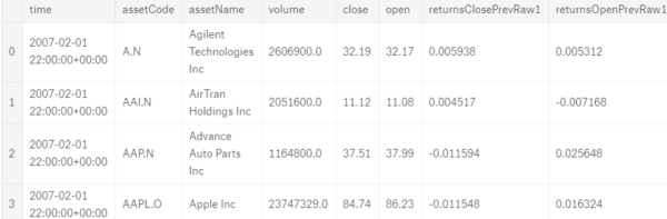
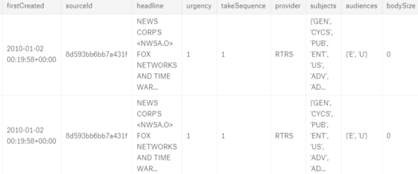
"market_train_df" is a dataframe that contains market information such as stock code, open price, close price, trading volume, etc. While "news_train_df" is a dataframe that stores stocks related news information, such as headline, tag, word counts, the probability of rather the news is positive or negative, etc..
Every data science challenge comes with a target to solve. What is the target in this challenge then? Since this challenge is about stock trading, in order to get rich, we have to predict the stock price in future. In this challenge, we are going to predict the probability of a stock going up or down in next 10 days.
EDA on Stock Trading
"A picture is worth a thousand words". That is why we always use EDA (Exploratory Data Analysis) to visualize our findings. First, let's take a look on our market training dataset. Since there are about 3800 stock codes in 2007 to 2016 date range, we pick 5 stock codes we have mentioned in CodeAStar blog previously for our EDA. So we have: Alphabet (Google), Amazon, Apple, eBay and Microsoft.
import plotly.graph_objs as go import plotly.offline as py py.init_notebook_mode(connected=True) data = [] stock_name_arr = ['Microsoft Corp', 'Amazon.com Inc', 'Alphabet Inc', 'Apple Inc', 'eBay Inc'] for stock_name in stock_name_arr: trace = go.Scatter( x = market_train_df.loc[market_train_df['assetName'] == stock_name]['time'].dt.strftime(date_format='%Y-%m-%d').values, y = market_train_df.loc[market_train_df['assetName'] == stock_name]['close'].values, name=stock_name ) data.append(trace) layout = go.Layout( title = "Stocks Price Chart", xaxis=dict( title='Date', rangeslider=dict(visible=True), type='date' ), yaxis=dict( title="Price (USD)", type='log', autorange=True ) ) fig = go.Figure(data=data, layout=layout) py.iplot(fig)
Here we go:
You may see something strange there on the chart, yes, the stock prices of Apple and eBay dropped vertically on 2 occasions.

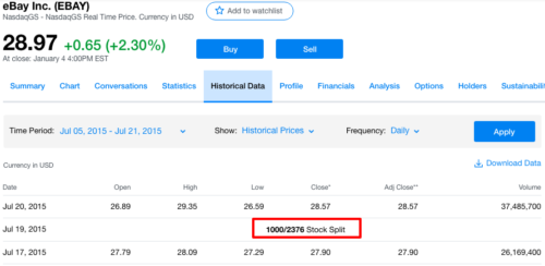
Don't panic. The stock data is fine without any error. As there were stock splits happened on both Apple and eBay stocks. The basic idea of stock split is, a corporation deciding to increase its total number of shares outstanding without altering the current market value.
We can go to Yahoo Finance to check stock split history of stocks.
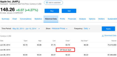
Luckily, the training dataset has already included the stock spilt data. Let's use Apple' stock price as our example:
market_train_df.loc[(market_train_df['time'] > '2014-06-05') & (market_train_df['assetCode'] == 'AAPL.O')]
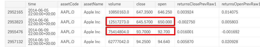
We can see the increase of volume and the drop of stock price within the dataset. So we do not need to do extra work for price adjustment in model training. But for visualization purpose, we can adjust the stock price according to its stock split ratio:
apple_adjusted = market_train_df.loc[market_train_df['assetName'] == 'Apple Inc'] ebay_adjusted = market_train_df.loc[market_train_df['assetName'] == 'eBay Inc'] apple_adjusted.loc[(apple_adjusted['time'] < '2014-06-09'), 'close'] = apple_adjusted.loc[apple_adjusted['time'] < '2014-06-09']['close']/7 ebay_adjusted.loc[(ebay_adjusted['time'] < '2015-07-20'), 'close'] = ebay_adjusted.loc[ebay_adjusted['time'] < '2015-07-20']['close']/2376*1000
And we have the updated chart:
It lets us know that stock price and volume are correlated in our dataset.
Find Outliers
Since we have ~3800 stocks in the 10 years dataset, there may be some extraordinary data. It is good to have a data integrity check. First, let's find stocks with more than 300% change in price within the same day.
market_train_df['price_diff'] = (market_train_df['close']market_train_df['open'])/market_train_df['open'] market_train_df.loc[(market_train_df['price_diff'] > 3) | (market_train_df['price_diff'] < -0.75)]
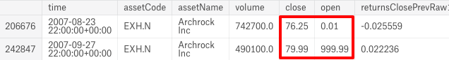
Then we find a stock with 0.01 opening price in one day and 999.99 opening price in another day. It should be some kind of data error.
We do the same checking on returnsClosePrevRaw1 and returnsOpenPrevRaw1, where returnsClosePrevRaw1 and returnsOpenPrevRaw1 are values storing the open or close price change ratio from previous day.
returnsClosePrevRaw1 = (Current Day Close Price - Previous Day Close Price) / Previous Day Close Price
returnsOpenPrevRaw1 = (Current Day Open Price - Previous Day Open Price) / Previous Day Open Price
And we remove those outliers from our dataset:
market_train_df= market_train_df.loc[market_train_df['returnsOpenPrevRaw1'].abs() <= 3] market_train_df= market_train_df.loc[market_train_df['returnsClosePrevRaw1'].abs() <= 3] market_train_df = market_train_df.loc[market_train_df['close']/market_train_df['open'] <= 3]
We also remove data earlier than 2010-01-01. This action is based on 2 reasons:
- to reduce memory usage as we can only use Kaggle's 17GB kernel in this challenge
- to skip the data dated in the 2008 global financial crisis period
news_train_df = news_train_df.loc[news_train_df['time'] >= '2010-01-01 22:00:00+0000']
On news_train_df dataframe, let' see rather we can find something useful there.
headtag_df = news_train_df.groupby(['headlineTag']).size().to_frame('count').reset_index().sort_values('count', ascending=False) trace = go.Bar( x = headtag_df['headlineTag'], y = headtag_df['count'] ) layout = go.Layout( title = "Headline Tag Count", xaxis=dict( title="Tag", tickangle=45, ), yaxis=dict( title="Count" ), ) data = [trace] fig = go.Figure(data=data, layout=layout) py.iplot(fig)
Most of the news has no headline tag and even existing tags are widely distributed, hardly provide important information to us. We should remove this feature when we build our machine learning model.
Build the Model
Since we are going to predict the stock trend, the objective of our model is to find the confidence of a stock going up or down in next 10 days (i.e. the returnsOpenNextMktres10 field). Before we start to build our model, first and foremost, we need to merge 2 training datasets "market_train_df" and "news_train_df", into one.
def mergeDF(market_df, news_df): market_df['time'] = market_df.time.dt.date market_df['returnsOpenPrevRaw1_to_volume'] = market_df['returnsOpenPrevRaw1'] / market_df['volume'] market_df['close_to_open'] = market_df['close'] / market_df['open'] market_df['average_price'] = (market_df['close'] + market_df['open'])/2 market_df['close_price_volume'] = market_df['volume'] * market_df['close'] news_df['firstCreated'] = news_df.firstCreated.dt.date news_df['time'] = news_df.time.dt.hour news_df['sentence_word_count'] = news_df['wordCount'] / news_df['sentenceCount'] news_df['assetCodesLen'] = news_df['assetCodes'].map(lambda x: len(eval(x))) news_df['assetCode_0'] = news_df['assetCodes'].map(lambda x: list(eval(x))[0]) news_df['headlineLen'] = news_df['headline'].apply(lambda x: len(x)) news_df = news_df.groupby(['firstCreated', 'assetCode_0'], as_index=False).mean() #merge market with news df market_df = pd.merge(market_df, news_df, how='left', left_on=['time', 'assetCode'], right_on=['firstCreated', 'assetCode_0']) #use left join, i.e. all depend on market df return market_df merged_train_df = mergeDF(market_train_df, news_train_df)
Our new dataset, merged_train_df, is grouped by the same date and the same stock code (assetCode). Since price is an important feature, we add new price features like average_price and close_price_volume.
After that we can start creating our training and validating datasets from our merged one. Remember, we are predicting stock prices' future trend, not their future value.
selected_cols = [c for c in market_train_df.columns if c not in ['time_x', 'assetCode', 'assetName', 'universe', 'firstCreated', 'assetCode_0', 'headlineTag', 'provider', 'time_y', 'returnsOpenNextMktres10']] train_x = market_train_df[selected_cols].values train_y = market_train_df.returnsOpenNextMktres10 >= 0 train_y = train_y.values from sklearn import model_selection X_train, X_test, Y_train, Y_test = model_selection.train_test_split(train_x, train_y, test_size=0.2, random_state=3)
Now we have training and validating datasets, it is time to make our training model. We can use basic parameters for our first model. But since we are predicting the price's up or down trend, we have to set our model objective to "binary".
import lightgbm as lgb params = {'learning_rate': 0.01, 'max_depth': 12, 'boosting': 'gbdt', 'objective': 'binary', 'metric': 'auc', 'seed': 33} model = lgb.train(params, train_set=lgb.Dataset(X_train, label=Y_train), num_boost_round=5000, valid_sets=[lgb.Dataset(X_train, label=Y_train), lgb.Dataset(X_test, label=Y_test)], verbose_eval=100, early_stopping_rounds=100)
After that we can sit and wait for our first training outcome.
Predict the Trend
Before we do the prediction, let's take a look on feature importance chart from our model.
impo_df = pd.DataFrame({'imp': model.feature_importance(), 'col':selected_cols}) impo_df = impo_df.sort_values(['imp','col'], ascending=[True, False]) colors=[] for i in range(len(selected_cols)): if i % 2 == 0: colors.append('#EFC62E') else: colors.append('#EF7D2E') data=[] trace = go.Bar( orientation = 'h', x = impo_df.imp, y = impo_df.col, marker=dict( color= colors, ) ) data.append(trace) layout = go.Layout( title = "Feature Importance Chart", titlefont=dict(size=25), xaxis=dict( title='Importance', titlefont=dict(size=20), ), yaxis=dict( title="Feature", tickangle=45, automargin=True, titlefont=dict(size=20), ) ) fig = go.Figure(data=data, layout=layout) py.iplot(fig)
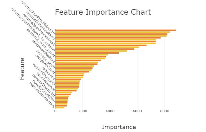
From the chart, we find that marketing features score higher in importance than news features.
We get the testing dataset using Kaggle's specified API, env.get_prediction_days(). Then we can predict the outcome in a date loop and submit to Kaggle.
days = env.get_prediction_days() start_time = time.time() for market_test_df, news_test_df, pred_template_df in days: market_test_df = mergeDF(market_test_df, news_test_df) #fill up with zero values X_live = market_test_df[selected_cols].values predictions = model.predict(X_live, num_iteration=model.best_iteration) confidence = 2 * predictions -1 preds_df = pd.DataFrame({'assetCode':market_test_df['assetCode'],'confidence':confidence}) pred_template_df['confidenceValue'][pred_template_df['assetCode'].isin(preds_df.assetCode)] = preds_df['confidence'].values env.predict(pred_template_df) print("Time used for prediction: {} seconds".format(time.time()-start_time)) env.write_submission_file()
Conclusion
Finally, our current model can score about 0.647 (mean divided by the standard deviation of daily confidence, the closer to 1 the better). It is definitely not helping us to get rich in stock market :]] . But, the main point of this exercise is, to learn the know-how on building our stock trading prediction model. So we summarize what we have experienced:
- market data is more important than news data
- price related features are important
- there may be outliers in training data
- there are global events which affect all stock prices in general
I would suggest we focus on price and volume features and apply certain day range patterns, in order to make good our model and get better result next time.
What have we learnt in this post?
- Feature engineering for stock trading datasets
- Data integrity on stock training datasets
- Handling on market news
- Stock prediction result criteria