Visualize a Convolutional Neural Network

On last post, we tried our image recognition project with handwritten digits. We used a Convolutional Neural Network (CNN) to train our machine and it did pretty well with 99.47% accuracy. We learnt how a CNN works by actually implementing a model. Today, we move one step further to learn more about the CNN, let's visualize our CNN in different layers!
Prepare our teaching material
When we learnt about Random Forest model, we used a project we did in past, the Titanic Survivors project, as our teaching material. So when we go to learn more about the CNN, we do the same thing again. This time, we use our last handwritten digits project.
First, we load the training dataset and required modules as usual.
import numpy as np import pandas as pd from keras.models import Sequential from keras.layers import Dense, Dropout, Flatten from keras.layers.convolutional import Conv2D, MaxPooling2D from keras.utils import np_utils from keras.optimizers import RMSprop from keras.callbacks import ReduceLROnPlateau import matplotlib.pyplot as plt from random import randrange df_train = pd.read_csv('../input/train.csv')
Then we define the same model as our previous project.
def cnn_model(result_class_size): model = Sequential() model.add(Conv2D(30, (5, 5), input_shape=(28,28,1), activation='relu')) model.add(MaxPooling2D(pool_size=(2, 2))) model.add(Conv2D(15, (3, 3), activation='relu')) model.add(Dropout(0.2)) model.add(Flatten()) model.add(Dense(128, activation='relu')) model.add(Dense(50, activation='relu')) model.add(Dense(result_class_size, activation='softmax')) model.compile(loss='categorical_crossentropy', optimizer=RMSprop(), metrics=['accuracy']) return model
We construct our model with training data and display the layer summary of our model.
df_train_x = df_train.iloc[:,1:] #get 784 pixel value columns after the first column df_train_y = df_train.iloc[:,:1] arr_train_y = np_utils.to_categorical(df_train_y['label'].values) model = cnn_model(arr_train_y.shape[1]) model.summary() _________________________________________________________________ Layer (type) Output Shape Param # ================================================================= conv2d_1 (Conv2D) (None, 24, 24, 30) 780 _________________________________________________________________ max_pooling2d_1 (MaxPooling2 (None, 12, 12, 30) 0 _________________________________________________________________ conv2d_2 (Conv2D) (None, 10, 10, 15) 4065 _________________________________________________________________ dropout_1 (Dropout) (None, 10, 10, 15) 0 _________________________________________________________________ flatten_1 (Flatten) (None, 1500) 0 _________________________________________________________________ dense_1 (Dense) (None, 128) 192128 _________________________________________________________________ dense_2 (Dense) (None, 50) 6450 _________________________________________________________________ dense_3 (Dense) (None, 10) 510 ================================================================= Total params: 203,933 Trainable params: 203,933 Non-trainable params: 0 _________________________________________________________________
Let's train our model with the training dataset. We just train it in 3 epochs for demonstration purpose.
df_train_x = df_train_x / 255 # normalize the inputs #reshape training X to (number, height, width, channel) arr_train_x_28x28 = np.reshape(df_train_x.values, (df_train_x.values.shape[0], 28, 28, 1)) model.fit(arr_train_x_28x28, arr_train_y, epochs=3, batch_size=100) Epoch 1/3 42000/42000 [==============================] - 38s 910us/step - loss: 0.2515 - acc: 0.9224 Epoch 2/3 42000/42000 [==============================] - 38s 895us/step - loss: 0.0711 - acc: 0.9790 Epoch 3/3 42000/42000 [==============================] - 37s 892us/step - loss: 0.0483 - acc: 0.9848
Visualize the CNN model
Prior to this section, we are just doing the similar thing like we did in our last project. But now, the magic starts here. We are going to visualize the CNN model.
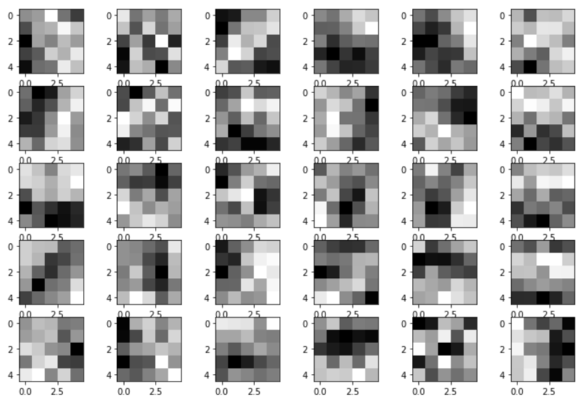
The first layer of our model, conv2d_1, is a convolutional layer which consists of 30 learnable filters with 5-pixel width and height in size. We do not need to define the content of those filters. As the model will learn building filters by "seeing" some types of visual feature of input images, such as an edge or a curve of an image. The 30 filters of our first layer should look like:
#get_weights [x, y, channel, nth convolutions layer ] weight_conv2d_1 = model.layers[0].get_weights()[0][:,:,0,:] col_size = 6 row_size = 5 filter_index = 0 fig, ax = plt.subplots(row_size, col_size, figsize=(12,8)) for row in range(0,row_size): for col in range(0,col_size): axundefined [col].imshow(weight_conv2d_1[:,:,filter_index],cmap="gray") filter_index += 1
In our first convolutional layer, each of the 30 filters connects to input images and produces a 2-dimensional activation map per image. Thus there are 30 * 42,000 (number of input images) = 1,260,000 activation maps from our first convolutional layer's outputs. We can visualize a output by using a random image from the 42,000 inputs.
test_index = randrange(df_train_x.shape[0]) test_img = arr_train_x_28x28[test_index] plt.imshow(test_img.reshape(28,28), cmap='gray') plt.title("Index:[{}] Value:{}".format(test_index, df_train_y.values[test_index])) plt.show()

Okay, the "7" digit image is our input. We then create a "display_activation" function to show the activation maps within a selected layer.
from keras.models import Model layer_outputs = [layer.output for layer in model.layers] activation_model = Model(inputs=model.input, outputs=layer_outputs) activations = activation_model.predict(test_img.reshape(1,28,28,1)) def display_activation(activations, col_size, row_size, act_index): activation = activations[act_index] activation_index=0 fig, ax = plt.subplots(row_size, col_size, figsize=(row_size*2.5,col_size*1.5)) for row in range(0,row_size): for col in range(0,col_size): axundefined [col].imshow(activation[0, :, :, activation_index], cmap='gray') activation_index += 1
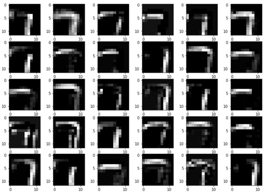
Then we display the 30 activation maps from the first layer in 6 columns and 5 rows.
display_activation(activations, 6, 5, 0)
Subsample the layer
Just after the execution of our first layer, there are already 1,260,000 activation map outputs. It is a common practice to apply a pooling layer. Thus we can subsample our outputs to reduce parameters and computation in our model. In our case, 2x2 pool size is used and works like following picture:
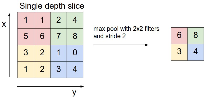
(image source: http://cs231n.github.io/convolutional-networks)
The image size is then drastically reduced. Since we only keep important data like the feature's existence rather than the feature's exact location, we can avoid overfitting.
To visualize the outputs of the pooling layer, we can use the "display_activation" function again with layer index set to 1 (the second layer, max_pooling2d_1).
display_activation(activations, 6, 5, 1)
The Expanding Network
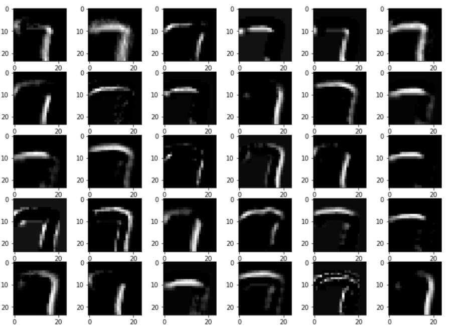
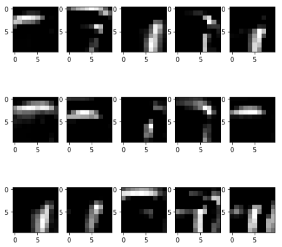
After the first 2 layers, we now have 1,260,000 inputs. On our 3rd layer, another convolutional layer, we are going to make 1,260,000 * 15 (number of filters) = 18,900,000 outputs. But don't panic, we only show one set of the activation maps here, i.e. 15 images. display_activation(activations, 5, 3, 2)

From the convolutional activation maps, we know that our model can now find features of a "7" like a horizontal stroke, a vertical stroke and a joining of strokes. We apply a dropout layer as our 4th layer to reduce overfitting. The dropping rate is set to 0.2, i.e. one input would be removed for every 5 inputs.
display_activation(activations, 5, 3, 3)
The purpose of dropout layer is to drop certain inputs and force our model to learn from similar cases. The result would be more obvious in a larger network.
Classification in Final Layer
We put outputs from the dropout layer into several fully connected layers. Our model then classifies the inputs into 0 - 9 digit values at the final layer. act_dense_3 = activations[7]
y = act_dense_3[0]
x = range(len(y))
plt.xticks(x)
plt.bar(x, y)
plt.show()
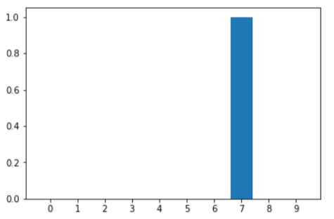
And we got the answer, "7".
What have we learnt in this post?
- how filters in a CNN be constructed
- visualization of a convolutional layer
- creation of a pooling layer