Python Image Recognizer with Convolutional Neural Network


On our data science journey, we have solved classification and regression problems. What's next? There is one popular machine learning territory we have not set feet on yet --- the image recognition. But now the wait is over, in this post we are going to teach our machine to recognize images by using Convolutional Neural Network (CNN).
Before we go further to our topic on Convolutional Neural Network, let's talk about another related term we will see often: Deep Learning.
Deep Learning is a subfield of machine learning which its model consists of multiple layers. The concept of a deep learning model is to use outputs from the previous layer as inputs for the successive layer. The model starts learning from the first layer and use its outputs to learn through the next layer. Eventually, the model goes "deep" by learning layer after layer in order to produce the final outcome.
Convolutional Neural Network is a type of Deep Learning architecture. We will use the abbreviation CNN in the post. Please don't mix up this CNN to a news channel with the same abbreviation. :]]
What is a Convolutional Neural Network?
We will describe a CNN in short here. For in depth CNN explanation, please visit "A Beginner's Guide To Understanding Convolutional Neural Networks". This is the best CNN guide I have ever found on the Internet and it is good for readers with no data science background.
Since a CNN is a type of Deep Learning model, it is also constructed with layers. A CNN starts with a convolutional layer as input layer and ends with a classification layer as output layer. There are multiple hidden layers in between the input and output layers, such as convolutional layers, pooling layers and fully connected layers. So a typical CNN model should look like:
Conv (Input) -> Pool -> Conv -> Pool -> FC -> FC (Output) Conv: convolutional layer Pool: pooling layer FC: fully connected layer
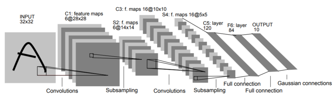
(image source: http://yann.lecun.com/exdb/publis/pdf/lecun-98.pdf)
Feel dizzy for seeing different layers? Don't worry, we can have short explanations on each layer here. For in-depth details, please refer to the CNN guide I mentioned previously.
- Convolutional Layer: a layer to store local conjunctions of features from the previous layer
- Pooling Layer: a layer to reduce the previous layer' size by discarding less significant data
- Fully Connected Layer: a layer have full connections to all activations in the previous layer
CNN in action
I always believe the best way to learn something is to do something. When we started to learn our first ever machine learning project, we do the "Hello World" way, by coding the iris classification. For image recognition and deep learning, the "Hello World" project for us is, the MNIST Database of Handwritten Digits.
This is a dataset of handwritten digits, our objective is to train our model to learn from 42,000 digit images, and recognize another set of 28,000 digit images. Before we actually start our project, we need to install our python deep learning library, Keras. Please note that deep learning requires relatively large processing resources and time. If this is your concern, I would suggest you to start a kernel from Kaggle Kernels for the deep learning project. As related libraries and datasets have already installed in Kaggle Kernels, and we can use Kaggle's cloud environment to compute our prediction (for maximum 1 hour execution time). As long as we have internet access, we can run a CNN project on its Kernel with a low-end PC / laptop. Once the preparation is ready, we are good to set feet on the image recognition territory.
The line starts here
First, let's import required modules here. We will discuss those models while we use it in our code segments. from keras.models import Sequential from keras.layers import Dense, Dropout, Flatten from keras.layers.convolutional import Conv2D, MaxPooling2D from keras.utils import np_utils from keras.optimizers import RMSprop from keras.callbacks import ReduceLROnPlateau from keras.preprocessing.image import ImageDataGenerator import matplotlib.pyplot as plt from sklearn.model_selection import train_test_split from random import randrange We load training and testing data sets (from Kaggle) as usual. df_train = pd.read_csv('../input/train.csv') df_test = pd.read_csv('../input/test.csv') And take a look on the first 5 rows of the training data. df_train.head()
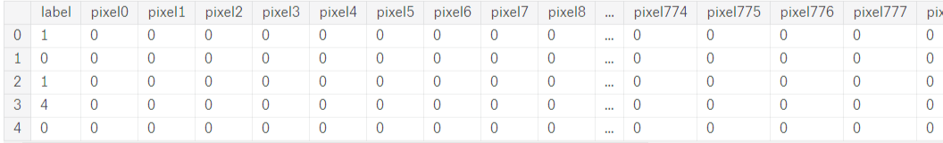
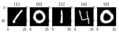
The first column "label" is the value of the hand written digit image. While the other 784 columns are the pixel values of a 28 width x 28 height (i.e. 784) gray-scale digit image. A picture is worth a thousand words, and now we are going to make 5 pictures, to visualize our first 5 digits from the testing data set.
df_train_x = df_train.iloc[:,1:] #get 784 pixel value columns after the first column df_train_y = df_train.iloc[:,:1] #get the first label column #reshape our training X into 28x28 array and display its label and image using imshow() ax = plt.subplots(1,5) for i in range(0,5): ax[1][i].imshow(df_train_x.values[i].reshape(28,28), cmap='gray') ax[1][i].set_title(df_train_y.values[i])
And the results are:
Libraries, check. Testing data, check. Now, it is the core part of our CNN project:
Build the Model
def cnn_model(result_class_size): model = Sequential() model.add(Conv2D(30, (5, 5), input_shape=(28,28,1), activation='relu')) model.add(MaxPooling2D(pool_size=(2, 2))) model.add(Conv2D(15, (3, 3), activation='relu')) model.add(Dropout(0.2)) model.add(Flatten()) model.add(Dense(128, activation='relu')) model.add(Dense(50, activation='relu')) model.add(Dense(result_class_size, activation='softmax')) model.compile(loss='categorical_crossentropy', optimizer=RMSprop(), metrics=['accuracy']) return model We use Conv2D() to create our first convolutional layer, with 30 features and 5x5 feature size. And the input shape is the shape of our digit image with height, width and channels. I.e. (28, 28, 1) Since all our digit images are gray-scale images, we can assign 1 to the channel. For color images, you need to assign 3 (R-G-B) to the channel. We activate the hidden layers with ReLU (rectified linear unit) activation. The concept of ReLU activation is quite straight forward, when there is an negative value on the hidden layer(feature can not be found on the input image), it returns zero, otherwise it returns the raw value.
After processing our first convolutional layer, there would be 30 more hidden layers per each digit image. We then use the pooling layer to down sample our layers, for every 2x2 area. Now we have smaller hidden layers as input images for our next convolutional layer. Likes the case we have done in our first convolutional layer, the second convolutional layer generates even more hidden layers for us. We then apply a dropout layer, which remove 20% units in our network to prevent overfitting.
At this moment, our CNN is still processing 2D matrix and we need to convert those units into 1D vector for the final outcome, so we apply a flatten layer here. And we are at the last few steps of our model building. We add 2 fully connected layers to form an Artificial Neural Network, which lets our model to classify our inputs to 50 outputs. Finally, we add the last fully connected layer with the size of output layer and softmax activation to squeeze the probability values of our outputs.
Our model is done!
Actually, it is not yet done. :]] We just need to do one more step, compile the model with following parameters: loss, metrics and optimizer. We assign Log Loss ("categorical_crossentropy" in Keras) as loss function to measure how good our model is, i.e. how well predicated digit values match actual digit values. And "accuracy" as metrics for performance evaluation. Then for the optimizer, which is an algorithm for our model to learn after its each running cycle. I picked RMSprop for its good performance in several trial runs.
We have finally built the CNN model, let's take a summary of our product. But before doing this, we need to define the size of the digit values. As a human, we know that the handwritten digits should be 0 to 9, i.e. the size of 10. From a machine's prospective, we need to send it the available outcomes (the dataframe df_train_y we created previously) and let it categorize the possible results in binary matrix. We then use the range of the output binary matrix as the size of our model's output layer.
arr_train_y = np_utils.to_categorical(df_train_y['label'].values) model = cnn_model(arr_train_y.shape[1]) model.summary() Layer (type) Output Shape Param # ================================================================= conv2d_1 (Conv2D) (None, 24, 24, 30) 780 _________________________________________________________________ max_pooling2d_1 (MaxPooling2 (None, 12, 12, 30) 0 _________________________________________________________________ conv2d_2 (Conv2D) (None, 10, 10, 15) 4065 _________________________________________________________________ dropout_1 (Dropout) (None, 10, 10, 15) 0 _________________________________________________________________ flatten_1 (Flatten) (None, 1500) 0 _________________________________________________________________ dense_1 (Dense) (None, 128) 192128 _________________________________________________________________ dense_2 (Dense) (None, 50) 6450 _________________________________________________________________ dense_3 (Dense) (None, 10) 510 ================================================================= Total params: 203,933 Trainable params: 203,933 Non-trainable params: 0 _________________________________________________________________
You might notice there are parameters in certain layers, they are trainable variables for our CNN model. On our first convolutional layer (conv2d_1), parameters are come from:
parameters = number of features * ( feature width * feature height ) + bias from feature map i.e. 30 * ( 5 * 5 ) + 30 = 780
Then on our second convolutional layer (conv2d_2), since inputs of this layer are the outputs of previous layer,
parameters = inputs from previous layer * number of features * ( feature width * feature height ) + bias from feature map i.e. 30 * 15 * ( 3 * 3 ) + 15 = 4065
More trainable parameters mean more computing needed and in machine learning territory, more calculation doesn't always mean getting better results. We are good at this setup currently, let' see how well our model can performance.
Train the model
We have prepared our model, it is time to put it in action. But first, let's gather our training material. #normalize 255 grey scale to values between 0 and 1 df_test = df_test / 255 df_train_x = df_train_x / 255
#reshape training X and texting X to (number, height, width, channel)
arr_train_x_28x28 = np.reshape(df_train_x.values, (df_train_x.values.shape[0], 28, 28, 1))
arr_test_x_28x28 = np.reshape(df_test.values, (df_test.values.shape[0], 28, 28, 1))
#validation package size = 8%
random_seed = 7
split_train_x, split_val_x, split_train_y, split_val_y, = train_test_split(arr_train_x_28x28, arr_train_y, test_size = 0.08, random_state=random_seed)
We normalize the gray scale data into [0 ... 1] values, so our CNN model can run faster. And since our CNN model use 2D matrix as input, we reshape our data into 28 x 28 2D matrix. We further separate 8% of testing data to validation data. Now we have prepared our data sets, there are two extra techniques we can apply to boost our model's performance.
Finding the proper learning rate
On our CNN model, the learning rate parameter help us to identify the local minima of loss. Different learning rates produce different loss by running different number of epochs:
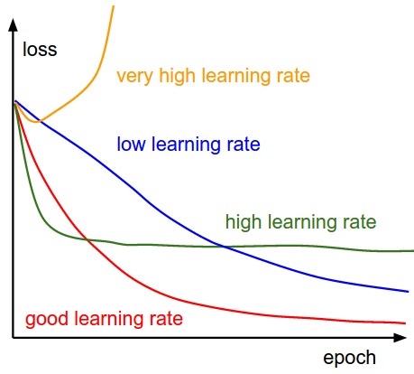
(image source: http://cs231n.github.io/neural-networks-3/)
We can manage the learning rate while we train our model, by using the ReduceLROnPlateau callback. In the following setting, we monitor the validation accuracy, reduce the learning rate by factor when there is no improvement after the number of patience (epochs):
reduce_lr = ReduceLROnPlateau(monitor='val_acc', factor=0.3, patience=3, min_lr=0.0001)
Self-Generated Images
Another technique we can apply is the use of image generator. The ImageDataGenerator from Keras can generate images from our inputs, randomly zoom, rotate and shift them horizontally and vertically. Thus we can have more testing images then the original testing dataset. datagen = ImageDataGenerator( rotation_range=10, zoom_range = 0.1, width_shift_range=0.1, height_shift_range=0.1) datagen.fit(split_train_x) Now, let's put all the things together. We train our model with testing and validation data sets, learning rate reducing callback and image generator in 30 rounds. model.fit_generator(datagen.flow(split_train_x,split_train_y, batch_size=64), epochs = 30, validation_data = (split_val_x,split_val_y), verbose = 2, steps_per_epoch=640, callbacks=[reduce_lr]) Similar results would prompt out: Epoch 1/30 - 37s - loss: 0.4305 - acc: 0.8626 - val_loss: 0.0861 - val_acc: 0.9735 Epoch 2/30 - 37s - loss: 0.1592 - acc: 0.9500 - val_loss: 0.0907 - val_acc: 0.9735
........
Epoch 29/30
- 39s - loss: 0.0342 - acc: 0.9898 - val_loss: 0.0199 - val_acc: 0.9929
Epoch 30/30 - 38s - loss: 0.0329 - acc: 0.9902 - val_loss: 0.0221 - val_acc: 0.9914
Our model is now well trained, we can obtain the prediction and save it in a csv file for submission. prediction = model.predict_classes(arr_test_x_28x28, verbose=0) data_to_submit = pd.DataFrame({"ImageId": list(range(1,len(prediction)+1)), "Label": prediction}) data_to_submit.to_csv("result.csv", header=True, index = False)
Since it is an image recognition project, why don't we validate our results by our own eyes?
We randomly pick 10 digit images from the testing dataset, then see rather our model can predict them right.
start_idx = randrange(df_test.shape[0]-10) fig, ax = plt.subplots(2,5, figsize=(15,8)) for j in range(0,2): for i in range(0,5): ax[j][i].imshow(df_test.values[start_idx].reshape(28,28), cmap='gray') ax[j][i].set_title("Index:{} \nPrediction:{}".format(start_idx, prediction[start_idx])) start_idx +=1
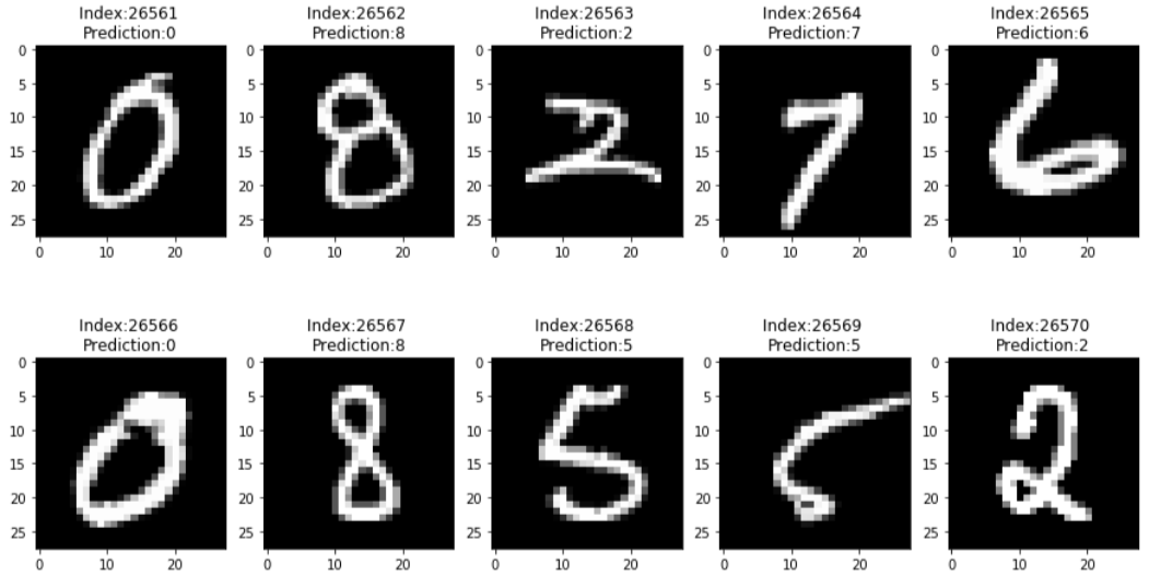
It looks good, doesn't it?
I submitted the result to Kaggle and scored 0.99471. By using the code on this post, it should be able to help you get at least 99.0% accuracy. Feel free to modify / enhance the code to get even better accuracy then.
What have we learnt in this post?
- Introduction of deep learning
- Introduction of convolutional neural network
- Use of learning rate control technique
- Use of image generation technique
The complete source code can be found at:
Kaggle Kernel: https://www.kaggle.com/codeastar/fast-and-easy-cnn-for-starters-in-keras-0-99471
GitHub: https://github.com/codeastar/digit-recognition-cnn