To win big in real estate market using data science - Part 2: Model Params Tuning


Previously on CodeAStar: A data alchemist wannabe tried to win big in real estate market, he then used Kaggle's Housing Regression data set, engineered the features and fit them in a bunch of models. Dang! Nothing fancy happened. But he then discovered "the room", the room for improvement --- model params tuning.
Enter the Model Params Tuning Room
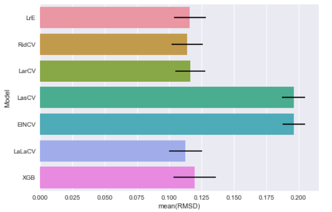
Before we enter "the room for improvement", let's rewind our models' scores from last post: [LinearRegression - LrE] Mean: 0.11596371 Std. Dev.: 0.012097 [Ridge - RidCV] Mean: 0.11388354 Std. Dev.: 0.012075 [Lars - LarCV] Mean: 0.11630241 Std. Dev.: 0.011665 [Lasso - LasCV] Mean: 0.19612691 Std. Dev.: 0.008914 [ElasticNet - ElNCV] Mean: 0.19630787 Std. Dev.: 0.008867 [LassoLars - LaLaCV] Mean: 0.11258596 Std. Dev.: 0.012750 [XGBoost - XGB] Mean: 0.11961144 Std. Dev.: 0.016610And the chart goes:
Since there is nothing else to tune in the Linear Regression model, we start our tuning journey on the Ridge model.
Ridge model is a regression model with L2 regularization, i.e. with the sum of square of coefficients. When we pass a stronger regularization parameter (alpha) to Ridge, it reduces feature variances and the model complexity, but causes underfitting. On the other hand, when we pass a smaller alpha parameter to Ridge, it trends to fit each deviation and causes overfitting. When we pass a 0 as alpha, it just becomes plain Linear Regression. So, how should we tune our Ridge model?
With great power comes great "regularization"
My Uncle Ben told me once.....
"@#%! Do you read CodeAStar web site? Why don't you use the K-Fold Cross Validation for model params tuning??"
Okay, just know that Uncle Ben is a loyal CodeAStar reader. Thank you Ben, let' start to use our good O' K-Fold Cross Validation.
We can reuse our code from previous post on the CV part and add a list of alpha parameter to Ridge:
kfold = KFold(n_splits=10) def getCVResult(models, X_learning, Y_learning): rmsds = [] for name, model in models: cv_results = cross_val_score(model, X_learning, Y_learning, scoring='neg_mean_squared_error', cv=kfold ) rmsd_scores = np.sqrt(-cv_results) print("\n[%s] Mean: %.8f Std. Dev.: %8f" %(name, rmsd_scores.mean(), rmsd_scores.std())) rmsds.append(rmsd_scores.mean()) return rmsds alphas = [0.00001, 0.00005, 0.0001, 0.0005, 0.005, 0.01, 0.05, 0.1, 0.5, 1, 1.5] models_R = [] for alpha in alphas: models_R.append(("Rid_"+str(alpha), Ridge(alpha=alpha) )) rmsds = getCVResult(models_R, X_learning, Y_learning)
And get following results:
[Rid_1e-05] Mean: 0.11348263 Std. Dev.: 0.012197 [Rid_5e-05] Mean: 0.11336354 Std. Dev.: 0.012281 [Rid_0.0001] Mean: 0.11333158 Std. Dev.: 0.012282 [Rid_0.0005] Mean: 0.11320434 Std. Dev.: 0.012232 [Rid_0.005] Mean: 0.11268473 Std. Dev.: 0.012124 [Rid_0.01] Mean: 0.11255269 Std. Dev.: 0.012144 <---[Rid_0.05] Mean: 0.11313334 Std. Dev.: 0.012147 [Rid_0.1] Mean: 0.11388355 Std. Dev.: 0.012075 [Rid_0.5] Mean: 0.11617453 Std. Dev.: 0.011926 [Rid_1] Mean: 0.11696996 Std. Dev.: 0.011962 [Rid_1.5] Mean: 0.11732840 Std. Dev.: 0.012024
Let's put our results in a data frame.
df_ridge = pd.DataFrame(alphas, columns=['alpha']) df_ridge['rmsd'] = rmsds sns.pointplot(x="alpha", y="rmsd", data=df_ridge) plt.show()
A picture is worth a thousand words (although I rarely post more than 1000 words here):
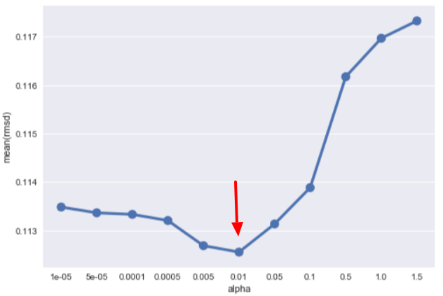
Let's back up, a larger alpha brings out underfitting and a smaller one brings out overfitting. When we apply the K-Fold CV, we can get the most suitable value we want.
The Lasso of Truth
Wonder Woman's golden lasso can make people confess and tell the truth. There is a "Lasso" model in data science, but it is nothing related to the Wonder Woman's weapon. Although it is no the Lasso of Truth, it does help us to get better prediction on our subjects.
Likes Ridge model, Lasso model is a regression model with regularization. But this time, it is L1 regularization, i.e. with the sum of absolute value of coefficients. Theoretically, Lasso should be a better model as it performs feature selection. It ignores features with zero coefficient to prevent overfitting. But, we don't have million features for Lasso to select. So it is no much difference for using either L1 or L2 regularization, at least in current data set.
We then do the same routine as Ridge model, by applying a set of alpha values, and let CV handle the rest:
alphas = [0.000001, 0.000005,0.00001, 0.00005, 0.0001, 0.0005, 0.001, 0.005, 0.01, 0.05, 0.1] models_las = [] for alpha in alphas: models_las.append(("Las_"+str(alpha), Lasso(alpha=alpha) ))
Here come the scores:
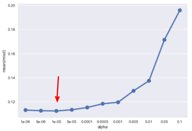
[Las_1e-06] Mean: 0.11310858 Std. Dev.: 0.012213 [Las_5e-06] Mean: 0.11258957 Std. Dev.: 0.011937 [Las_1e-05] Mean: 0.11238117 Std. Dev.: 0.011936 <---[Las_5e-05] Mean: 0.11334478 Std. Dev.: 0.012809 [Las_0.0001] Mean: 0.11526842 Std. Dev.: 0.012386 [Las_0.0005] Mean: 0.11833705 Std. Dev.: 0.012650 [Las_0.001] Mean: 0.11961042 Std. Dev.: 0.012739 [Las_0.005] Mean: 0.12906609 Std. Dev.: 0.012915 [Las_0.01] Mean: 0.13737188 Std. Dev.: 0.011742 [Las_0.05] Mean: 0.17137819 Std. Dev.: 0.008359 [Las_0.1] Mean: 0.19586111 Std. Dev.: 0.009045
Let's visualize the output again:
We then apply the same routine on ElasticNet and LassoLars models to find the best parameters:
#ElasticNet with alpha = 0.00001 and L1 ratio = 0.8 [ELN_L1_0.8] Mean: 0.11219824 Std. Dev.: 0.012191 #LassoLars with alpha = 0.000037 [LaLa_3.7e-05] Mean: 0.11207374 Std. Dev.: 0.012852
Cross Validation checks model's parameter one by one. What if we want to tune more than one parameter a time? No problem, we can use grid search in finding the best parameter combination.
Grid Search Tuning
Let' start our grid search tuning with XGBoost model. First, we get our estimator value from the Cross Validation method, i.e. n_estimators = 470. Then we try to find the best max_depth and min_child_weight values using GridSearchCV(). from sklearn.model_selection import cross_val_score, GridSearchCV
param_test =
{
'max_depth':[3,4,5,7],
'min_child_weight':[2,3,4]
}
gsearch = GridSearchCV(estimator = xgb.XGBRegressor(n_estimators=470),
param_grid = param_test, scoring='neg_mean_squared_error', cv=kfold)
gsearch.fit(X_learning,Y_learning)
print(gsearch.best_params_ )
print(np.sqrt(-gsearch.best_score_ ))
We put tuning parameters into param_test array and let GridSearchCV() do the validation job. The program will then print out the best parameter combination and the best RMSD score.{'max_depth': 3, 'min_child_weight': 3} 0.115714387592
Now we put n_estimators, max_depth and min_child_weight into XGBRegressor, and run CV to find the best gamma value.
gammas = [0.0002, 0.0003, 0.00035, 0.0004, 0.0005] models_xgb_gamma = [] for gamma in gammas: models_xgb_gamma.append(("XGB_"+str(gamma), xgb.XGBRegressor(n_estimators=470,max_depth=3, min_child_weight=3, gamma=gamma ) )) getCVResult(models_xgb_gamma, X_learning, Y_learning)
We pick the best result from CV:
[XGB_0.0003] Mean: 0.11366855 Std. Dev.: 0.012560
After that, we keep running GridSearchCV() and CV with other parameters: subsample, learning_rate, reg_alpha and reg_lambda. Thus, we can find the best parameter combination for XGBRegressor model.
It' Show Time
We have tuned our models, it is the time to see how it can improve our models' performances. tuned_models = [] tuned_models.append(("Rid_t", Ridge(alpha=0.01) )) tuned_models.append(("Las_t", Lasso(alpha=0.00001) )) tuned_models.append(("ElN_t", ElasticNet(l1_ratio=0.8, alpha=0.00001) )) tuned_models.append(("LaLa_t", LassoLars(alpha=0.000037) )) tuned_models.append(("XGB_t", xgb.XGBRegressor(n_estimators=470,max_depth=3, min_child_weight=3, learning_rate=0.042,subsample=0.5, reg_alpha=0.5,reg_lambda=0.8) ))
getCVResult(tuned_models, X_learning, Y_learning)
Here they come:[Ridge Tuned Rid_t] Mean: 0.11255269 Std. Dev.: 0.012144 [Lasso Tuned Las_t] Mean: 0.11238117 Std. Dev.: 0.011936 [ELasticNet Tuned ElN_t] Mean: 0.11233786 Std. Dev.: 0.011963 [LassoLars Tuned LaLa_t] Mean: 0.11231273 Std. Dev.: 0.012701 [XGBoost Tuned XGB_t] Mean: 0.11190687 Std. Dev.: 0.015171
With new chart:
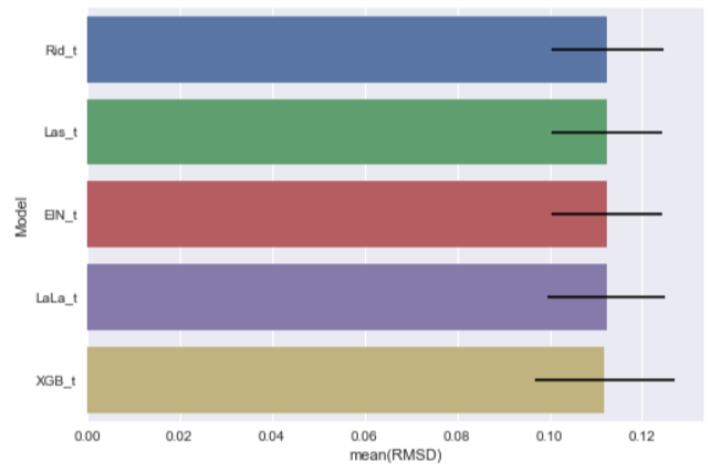
We find that all the tuned models perform better than before! We are getting closer and closer to the "room" for improvement.
But, there is something missing in our post. We have used CV and GridSearchCV for getting the best parameters, however other than the alpha parameter, the detail of each parameter is omitted. What is going on here? Well, we will leave this topic to next post, the final chapter of our housing regression model trilogy :]] .
What have we learnt in this post?
- Apply model params tuning can get better prediction
- Use cross validation for getting the best single parameter in a model
- Use GridSearchCV() method for getting the best combination among parameters