RNN (Recurrent Neural Network) in NLP and Python – Part 2

From our Part 1 of NLP and Python topic, we talked about word pre-processing for a machine to handle words. This time, we are going to talk about building a model for a machine to classify words. We learned to use CNN to classify images in past. Then we use another neural network, Recurrent Neural Network (RNN), to classify words now.

What is Recurrent Neural Network (RNN)?

RNN is a class of deep neural networks and so is the CNN. Then what is the major difference between CNN and RNN? The spelling. (okay, don’t laugh, I’m serious :]] ) The “R” of RNN stands for Recurrent. It means process is occupied repeatedly and this is the feature we don’t see in CNN.

In CNN, we call it a feed-forward network. While the input of layer 2 is the output of layer 1, the input of layer 3 is the output of layer 2 and the list goes on. But in RNN, things go repeatedly, as the inputs of layer 2 are the output of layer 1 and also the output of layer 2. A RNN not only produces output, it can copy and loop it back to the network. It turns out RNN is a neural network with memory.

It also makes RNN strong on handling sequence of data to predict precise outcome. The content of sequential data, e.g. speech, depends on how data is connected. When we have “Have”, “a” and “nice” as inputs, RNN remembers those inputs and predict “day” as output. That is also why RNN is widely used on text recognition and translation applications. We can explain a RNN with following diagram:

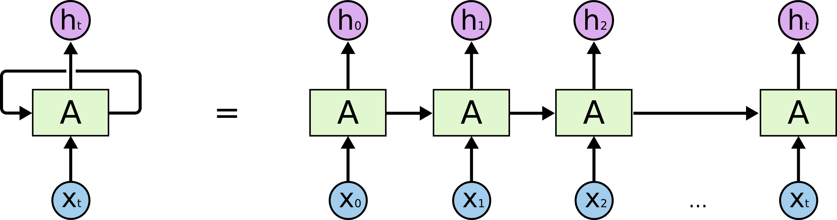
First, an input, X_t, passes through RNN, A. It starts from the first round. We call the first chunk of input as X_0. RNN then produces hidden output h_0. Then we go for the next round with input X_1, h_0 is added to the RNN, and we have hidden output h_1. The flow goes again and again until we put all our input into A. Finally, we have h_t as our output which trains with previous inputs.

RNN in Python

From our Python Image Recognizer post, we built a CNN model for image classification with Keras. This time, we are going to use the Keras library again, but for a RNN model. Firstly, let’s import required modules.

from keras.preprocessing.text import Tokenizer
from keras.preprocessing.sequence import pad_sequences
from keras.layers import Embedding, Input, Dense, CuDNNLSTM, concatenate, Bidirectional, SpatialDropout1D, Conv1D, GlobalAveragePooling1D, GlobalMaxPooling1D
from keras.optimizers import Adam
from keras.models import Model
from keras.callbacks import EarlyStopping, ModelCheckpoint
import keras.backend as K
from sklearn.model_selection import KFold

Then we apply the word pre-processing function, punct_apo_fix, from Part 1 and pre-process our training and testing data.

df_merge = pd.concat([df_train[['id','comment_text']], df_test], axis=0)
df_merge["comment_text"] = df_merge["comment_text"].apply(lambda x: punct_apo_fix(x))
df_train_comment = df_merge.iloc[:df_train.shape[0],:]
df_test_comment = df_merge.iloc[df_train.shape[0]:,:]
df_train_comment = pd.concat([df_train_comment,df_train[['target']]],axis=1)

Now we normalize our training data and get the word vector indexes from the pre-trained fastText model.

df_train_comment['target'] = np.where(df_train_comment['target'] >= 0.5, True, False)
tokenizer = Tokenizer(num_words=100000)
tokenizer.fit_on_texts(list(df_train_comment['comment_text']) + list(df_test_comment['comment_text']))
total_unique_word = len(tokenizer.word_index) + 1
wordvectors_index = KeyedVectors.load_word2vec_format(fasttext_300d_2m_model)

Next, we apply the fastText word vector indexes into words found from our training and testing data.

EMBEDDINGS_DIMENSION = 300
embedding_matrix = np.zeros((total_unique_word,EMBEDDINGS_DIMENSION))
for word, i in tokenizer.word_index.items():
    if word in wordvectors_index.vocab:
        embedding_matrix[i] = wordvectors_index[word]

Okay, we are going to the fun part of this project — build the model!

RNN model with LSTM and Bidirectional Structure

Before we start to build our model, there are 2 techniques we can apply on RNN to make good the model. They are Long Short-Term Memory (LSTM) and Bidirectional RNN. Let’ start with LSTM first.

When our input data is “People in Japan speak… “. We can expect the output should be “Japanese” from our human’s mind. But from a machine’s perspective, it does not have enough information to generate the output. It needs the relationship of “Japan” and “Japanese” from other inputs. That is why we need LSTM to extend RNN memory for not only current input but also previous inputs.

Then we go for the Bidirectional RNN. The concept of Bidirectional structure is straight-forward. It duplicates a recurrent layer but in reverse order. When we have “Have a nice day.” as input, it will turn out becoming 2 layers with “Have“, “a“, “nice“, “day“, “.” and “.“, “day“, “nice“, “a“, “Have“. So what is the benefit of using Bidirectional structure? Let’s think about “We go to a __________ to have lunch there“. The RNN reads “We“, “go” “to” forwardly and “there“, “lunch“, “have” backwardly. Then it can predict “restaurant” by relating inputs from the 2 layers.

Now we put those techniques into our model:

MAX_SEQUENCE_LENGTH = 256
def build_model(total_unique_word, embedding_matrix):
    sequence_input = Input(shape=(MAX_SEQUENCE_LENGTH,), dtype='int32')
    embedding_layer = Embedding(total_unique_word,
                            EMBEDDINGS_DIMENSION,
                            weights=[embedding_matrix],
                            input_length=MAX_SEQUENCE_LENGTH,
                            trainable=False)
    x = embedding_layer(sequence_input)
    x = SpatialDropout1D(0.2)(x)
    x = Bidirectional(CuDNNLSTM(64, return_sequences=True))(x)   
    x = Conv1D(64, kernel_size = 2, padding = "valid", kernel_initializer = "he_uniform")(x)
    avg_pool1 = GlobalAveragePooling1D()(x)
    max_pool1 = GlobalMaxPooling1D()(x)     
    x = concatenate([avg_pool1, max_pool1])
    preds = Dense(1, activation='sigmoid')(x)
    model = Model(sequence_input, preds)
    model.compile(loss='binary_crossentropy',
              optimizer=Adam(),
              metrics=['acc'])
    return model

As we mentioned in Part 1, a machine handles words using word vectors. That is why we apply Embedding layer to convert input to vector. And you may notice that, instead of using Droupout layer, we use SpatialDropout1D. It will drop entire 1D feature maps, and make bigger difference for machine to learn.

Predict Comment Classification

Data pre-processing, check. Model building, check. Now it is the time we go for predicting those comments are toxic or not. We also apply 3-fold cross validation to enhance our prediction.

train_text = pad_sequences(tokenizer.texts_to_sequences(df_train_comment["comment"]), maxlen=MAX_SEQUENCE_LENGTH)
test_text = pad_sequences(tokenizer.texts_to_sequences(df_test_comment["comment"]), maxlen=MAX_SEQUENCE_LENGTH)
train_target = df_train_comment["target"]
n_splits=3
splits = list(KFold(n_splits).split(train_text,train_target))
test_preds = np.zeros((df_test_comment.shape[0]))
for fold in list(range(n_splits)):
    K.clear_session()
    tr_ind, val_ind = splits[fold]
    checkpoint = ModelCheckpoint(f'gru_{fold}.hdf5', save_best_only = True)
    earlystop = EarlyStopping(monitor='val_loss', mode='min', verbose=1, patience=3)
    model = build_model()
    model.fit(train_text[tr_ind],
        train_target[tr_ind],
        batch_size=2048,
        epochs=100,
        validation_data=(train_text[val_ind], train_target[val_ind]),
        callbacks = [earlystop,checkpoint])
    test_preds += model.predict(test_text)[:,0]
test_preds /= n_splits
submission = pd.read_csv('../input/jigsaw-unintended-bias-in-toxicity-classification/sample_submission.csv', index_col='id')
submission['prediction'] = test_preds
submission.reset_index(drop=False, inplace=True)

After around 2 hours processing time, we have the prediction and we can discover how well a machine can do for a human’s work.

validation_df = pd.merge(test_df, submission, on='id')
validation_df[validation_df.prediction > 0.5].head()
validation_df[validation_df.prediction < 0.5].head()

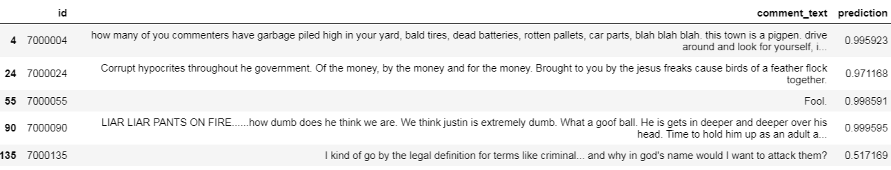
This is a group of machine classified toxic comments:

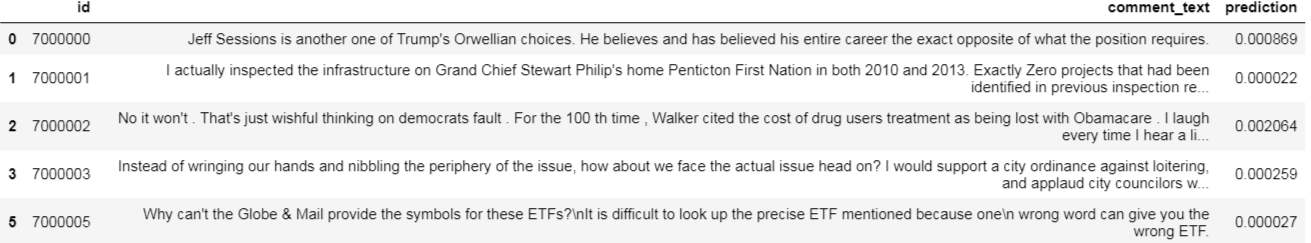
And this is a group of non-toxic comments:

I do not have any issue for non-toxic comments, just the toxic comments part is a bit, "high moral standard" :]] .

When I submit above prediction to Kaggle, it turns out scoring 0.92x , i.e. 92.x% accuracy. There is still room for improvement, keep trying and learning!

What have we learnt in this post?

1. Definition of Recurrent Neural Network
2. Concept of LSTM
3. Concept of Bidirectional structure
4. Building RNN model in Python