Word Embedding in NLP and Python – Part 1

We have handled text in machine learning using TFIDF. And we can use it to build word cloud for analytic purpose. But is it the capability of a machine can do on text? Definitely not, as we just haven’t let machine to “learn” about text yet. TFIDF is a statistics process, while we want a machine to learn the correlation of text. So a machine can read and understand texts like a human does, we call it Natural Language Processing (NLP). We can think about that, we teach TFIDF to a machine in a Mathematics class. This time, we teach a machine in a Linguistics class. And our first lesson will be — word embedding.

Word in machine’s POV

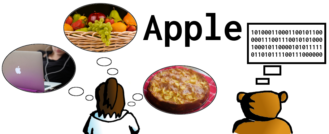
When we read a word, “apple”, we may think of a reddish fruit, a pie ingredient or even a technology company. We have such thinking because we have learnt from class or experienced from our daily life. For a machine, “apple” is just a five-character length word. In fact, it is a bunch of 0 and 1 from a machine’s point of view.

Our work is helping a machine to learn the correlation of words. So we let words attach with other words — that is why we call it the “word embedding”.

How word embedding works in a machine

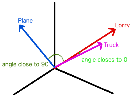
Now we know what to do for machine learning on text. It is time to understand how do we achieve our goal. As we mentioned earlier, a machine treats words as a bunch of 0 and 1. The first thing we do is to encode words into vectors, i.e. each word has its geometric location. The next thing we do is to bind words with similar context into close geometric locations. Mathematically, the cosine of the angle between those vectors should be close to 1 and the angle should be close to 0. Let’ see following example, we have 3 different words, “Lorry”, “Truck” and “Plane”. Our objectives are letting machine has similar words in close position, and has unmatched word in far position.

Word Embedding technology #1 – Word2Vec

In order to do word embedding, we will need Word2Vec technology on neural networks. Word2Vec was developed by Tomas Mikolov and his teammates at Google. It consists of two methods, Continuous Bag-Of-Words (CBOW) and Skip-Gram.

CBOW is the way we predict a result word using surrounding words. For example, “day” is the predicted word, when our bag-of-words inputs are “Have”, “a”, “nice”. And “nice” is the predicted one when our inputs are “Have”, “a”, “day”.

On the other hand, Skip-Gram is a reverse of CBOW. We start our prediction from our target word, and calculate the possibility of its surrounding words.

Word Embedding technology #2 – fastText

After the release of Word2Vec, Facebook’s AI Research (FAIR) Lab has built its own word embedding library referring Tomas Mikolov’s paper. So we have fastText library. The major difference of fastText and Word2Vec is the implementation of n-gram. We can think of n-gram as sub-word. FastText breaks a word into several 3-4 characters length n-grams. For example, “action“, fastText will handle it as “<ac”, “act”, “cti“, “tio”, “ion“, “on>. Please note that “<” and “>” are added to the first-gram and the last-gram. So a machine can distinguish shorter words and other n-grams. Likes the word “act“, is “<act>” from a machine’s POV, not the n-gram “act“.

NLP in action

I believe practicing with example is a good way of learning. And it is always good to code something in CodeAStar here :]] . This time, we use a Kaggle’s competition topic, Toxicity Classification, as our NLP example. In the competition, our goal is to find out toxic comments, i.e. comments with vulgar or insulting languages.

Now we know that we must train a machine with texts first, so it can correlate what words are toxic and non-toxic. We can pick one of those embedding technologies and start to train a machine with training data.

When we learn a common language, in this case, English, we know some words are correlated and some are not. And we should not have much difference in general, otherwise we cannot communicate with each other. Then we apply this case to a machine. Each machine should has same word embedding vectors when each of them use the same technology and the same training data.

That’s it. We can use the pre-trained word embedding model instead of training ourselves. From fastText official website, we can download the pre-trained model which fastText used 600 billion tokens (“words”) to make 300 million vectors (“unique words”) from Common Crawl. It is a good way to save our time and effort. And most importantly, I don’t think I have a powerful machine to train with 600 billion tokens. :]]

Load the Pre-Trained Model

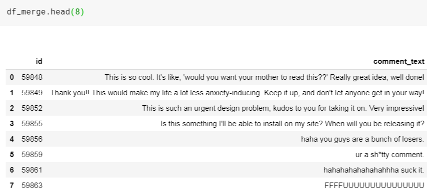
Okay, we first load the Kaggle’s training and testing data which contain toxic/non-toxic comments. Then we merge them together as a data frame, df_merge.

import pandas as pd
df_train = pd.read_csv('../input/jigsaw-unintended-bias-in-toxicity-classification/train.csv')
df_test = pd.read_csv('../input/jigsaw-unintended-bias-in-toxicity-classification/test.csv')
df_merge = pd.concat([df_train[['id','comment_text']], df_test], axis=0)

Let’ see what’s inside the data frame:

Our objective is changing the words in our comments into word vectors. So we load the word vectors from fastText pre-trained model using Gensim’s KeyedVectors library.

from gensim.models import KeyedVectors
fasttext_300d_2m_model = '../input/fasttext-crawl-300d-2m/crawl-300d-2M.vec'
wordvectors_index = KeyedVectors.load_word2vec_format(fasttext_300d_2m_model)

Now we have 2 million word vectors, but is it large enough to cover the words in our comments? And what are those words that we cannot find in our word vectors? Don’t worry, let’s find it out. Firstly, we discover the unique words (vocabulary list) from our comments.

from tqdm import tqdm
def build_vocab(texts):
    sentences = texts.apply(lambda x: x.split()).values
    vocab = {}
    for sentence in tqdm(sentences):
        for word in sentence:
            try:
                vocab[word] += 1
            except KeyError:
                vocab[word] = 1
    return vocab

vocab = build_vocab(df_merge['comment_text'])
print(f"The length of vocab: {len(vocab)}")

100%|██████████| 1902194/1902194 [00:32<00:00, 58340.85it/s]
The length of vocab: 1731089

Wow, we have 1.73 million unique words and 2 million word vectors. The next things we do are to check our word vector coverage and find the “out of vocabulary” (oov) words.

def check_coverage(vocab,embeddings_index):
    a = {}
    oov = {}
    k = 0
    i = 0
    for word in tqdm(vocab):
        try:
            a[word] = embeddings_index[word]
            k += vocab[word]
        except:
            oov[word] = vocab[word]
            i += vocab[word]
            pass
    print('Found embeddings for {:.2%} of vocab'.format(len(a) / len(vocab)))
    print('Found embeddings for {:.2%} of all text'.format(k / (k + i)))
    sorted_x = sorted(oov.items(), key=operator.itemgetter(1))[::-1]
    return sorted_x

oov = check_coverage(vocab,wordvectors_index)

100%|██████████| 1731089/1731089 [00:06<00:00, 286005.84it/s]
Found embeddings for 16.91% of vocab
Found embeddings for 91.37% of all text

Oh well, something doesn’t feel right. We have only 16.9% of vocabularies with word vectors.

Let’ see what are those top 10 oov words:

oov[:10]

[("Trump's", 24673),
 ("aren't", 21696),
 ("Don't", 20822),
 ("wouldn't", 20611),
 ('Yes,', 20040),
 ("wasn't", 19084),
 ("You're", 14486),
 ("Let's", 14392),
 ('So,', 13755),
 ('it?', 12927)]

Got it! We have to deal with punctuation and apostrophes.

Word Preprocessing

We make a punct_apo_fix function to replace and separate punctuation and apostrophes in our comments.

import re
def punct_apo_fix(x):
    x = str(x)
    x = x.replace("_"," ")    
    for punct in "`’":
        x = x.replace(punct,"'")    
    for punct in '!,?()%":.$“/;#+*=>[]&-':
        x = x.replace(punct, f' {punct} ')
    apos = re.findall("'.*?[\s]", x)
    for apo in apos: 
        if apo.lower() in ["'t ","'re ", "' ", "'ve ", "'s ", "'ll ", "'d ", "'n ", "'clock ", "'m "]:
            x = x.replace(apo, f' {apo}')
        else:
            x = x.replace(apo, f" ' {apo[1:]}")
    if (x.endswith("'")): 
        x = x[:-1]+" '"        
    return x

After that, we apply our function to df_merge. Then we can check the coverage again.

df_merge["comment_text"] = df_merge["comment_text"].apply(lambda x: punct_apo_fix(x))
vocab = build_vocab(df_merge['comment_text'])
oov = check_coverage(vocab,wordvectors_index)

Wow! That is an improvement. And we have changed the coverage of unique words from 16.9% to 56.6%. Moreover, now we have 99.7% of all words covered. That means the uncovered 43.4% unique words are only the 0.3% of total words there.

We have a pre-processed data set, so the next thing we do, is to build our deep learning model. Stay tuned for the NLP in Python part 2.

What have we learnt in this post?

1. Definition of Word Embedding
2. Concept of Word2Vec
3. Concept of fastText
4. Usage of pre-trained model on word embedding
5. Usage of word pre-processing in NLP