U-Net and IoU for Object Detection in Image Processing
Other than our last
hand writing challenge ,there is another
Kaggle challenge featuring image recognition -- TGS Salt Identification Challenge . But this time, we are going for an "upgrade". As we are dealing with object detection. It is all about salt. In this challenge, our mission is finding geophysical images that contain salt. Oh wait, does it sound weird? Actually not. Salt in soil is bad on plant growth and can damage underground infrastructure like pipes and blocks. Salt identification can locate problematic parts, thus people can avoid or apply fix on those areas. Unlike the lasthand writing challenge
which we needed to find "what" the features were. This time, other than the "what", we need to find "where" the features are. And the good thing for this challenge is, new requirement comes new knowledge, so we have new knowledge to learn -- U-Net and IoU.Understand the Problem
Like all our previous Data Science projects, the first thing we do is to understand the problem. So we take a look on training data files from Kaggle. There are 2 folders, "images" and "masks". "Images" is a folder containing input images, while "masks" is a folder containing result images, i.e. where the salt is. We can visualize the training set in following lines of code: train_image_path = "../input/train/images/" train_mask_path = "../input/train/masks/"
image_array = []
for root, dirs, files in os.walk(train_image_path):
image_array = files
col_size = 7
row_size = 2
rand_id_array = random.sample(range(0, len(image_array)), col_size)
fig, ax = plt.subplots(row_size, col_size, figsize=(20,6))
for row in range(0,row_size):
image_index = 0
if (row==0):
da_path= train_image_path
else:
da_path= train_mask_path
for col in range(0,col_size):
img = load_img(da_path+image_array[rand_id_array[image_index]])
axundefined [col].imshow(img)
axundefined [col].set_title(image_array[rand_id_array[image_index]])
image_index += 1
plt.show()
We load 14 images randomly from the training set, the first 7 of them are input images and the last 7 are the salt mask images.
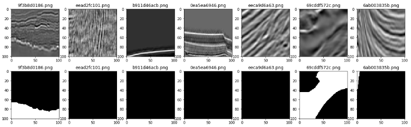
The input images are taken from somewhere in our Earth (Kaggle didn't expose the location[s]) and the mask images are showing where the salt is (the white part). Our goal is making mask images from testing data. Now our goal is clear, let's move to our next usual step in data science projects:
Features Engineering
First, we set the image to grayscale and divid it by 255. Thus image channel can be normalized within 0 to 1 range. df_train = pd.DataFrame({'id':train_id_arr,'image_path':train_image_arr,'mask_path':train_mask_arr})
df_train["image_array"] = [np.array(load_img(path=file_path, color_mode="grayscale")) / 255 for file_path in tqdm(df_train.image_path)]
df_train["mask_array"] = [np.array(load_img(path=file_path, color_mode="grayscale")) / 255 for file_path in tqdm(df_train.mask_path)]
Second, we calculate the coverage of each image and mask pair.img_width, img_height = img.size df_train["coverage"] = df_train.mask_array.map(np.sum) / (img_width * img_height)
For mask image with more salt (larger white area), the coverage value will trend to be closer to 1. On the other hand, the coverage value will be closer to 0 when there is no much salt (mostly dark in a mask image).
sns.distplot(df_train.coverage, kde=False)
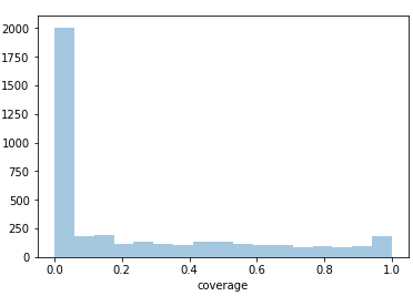
It is obvious that most of our images are salt-less. Now, we can categorize images into "coverage class" according to their "coverage" value.def cov_to_class(val): for i in range(0, 11): if val * 10 <= i : return i df_train["coverage_class"] = df_train.coverage.map(cov_to_class)
We are in the last step of our features engineering -- image resizing. Since we are going to use U-net architecture for object detection, we will resize our image from its original size 101 x 101 to 128 x 128, i.e. size with the power of 2.
targe_width = 128 targe_height = 128 def upsample(img_array): return resize(img_array, (targe_width, targe_height), mode='constant', preserve_range=True)
Entering the U-Net
We are about to build our learning model, the U-Net. But before doing this, we would like to prepare our training and validation datasets first. X_train, X_valid, Y_train, Y_valid = train_test_split( np.array(df_train.image_array.map(upsample).tolist()).reshape(-1, targe_width, targe_height, image_channel),#get a image array from df, upsample it np.array(df_train.mask_array.map(upsample).tolist()).reshape(-1, targe_width, targe_height, image_channel), #and reshape it to (unknown[image count], upsample_w, upsample_h, 1[channel]) test_size=0.2, stratify=df_train.coverage_class, random_state=256) We have 4000 pairs of training images and split 20% of them as validation data, i.e. 3600 pairs as training data, 800 pairs as validation data. You may notice that we use "stratify=df_train.coverage_class" to split the images. Thus data is split in a classified fashion, according to the "coverage_class". We apply this rule to ensure we have validation data in each class, otherwise the validation might be filled with the most dominated "class 0" data.
Now we are going to the core of this Data Science project -- build the U-Net model! But first things first, what is the U-Net?
The U-Net is a convolutional neural network (CNN) which it finds features from inputs and provides classifications. It is similar to the model we built in our hand writing recognition project. But, it is also a fully convolutional network (FCN). That means there is no dense / flatten layer and the model is connected layer by layer. From our hand writing project experience, we used convolutional and pooling layers to find image features and skipped the feature positions. In the U-Net architecture, we are going to get the feature locations as well. So we have transposed convolutional layers. Too many jargons? Let's have a simpler version: In the U-Net, we use downsampling for getting features, then we use upsampling for getting positions. The U-Net should look like:
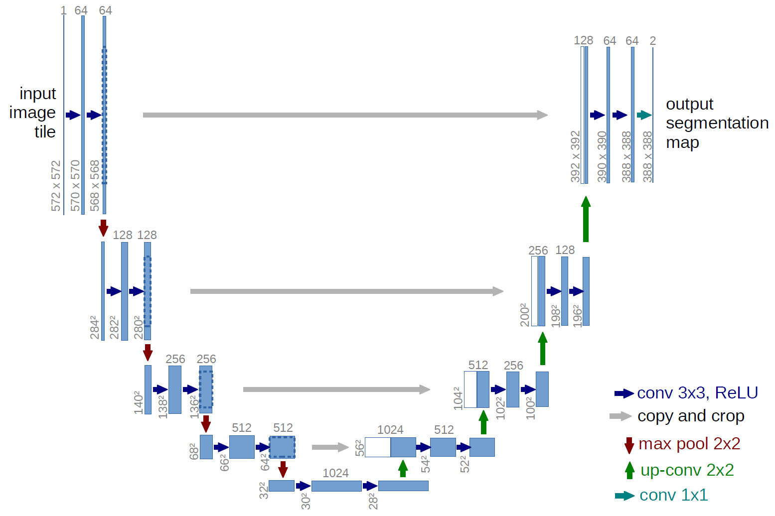
(image source: Dept. of Computer Science, University of Freiburg, Germany )
There are downsampling on the left side, upsampling on the right side and concatenating at the bottom. These setups make a U shaped architecture, that is why U-Net is the "U"-Net. :]]
DownSampling and UpSampling in U-Net
We should be no stranger with down sampling as we did taste it in the image recognition project before. We used the down sampling to locate features of hand writing digits.
(DownSampling from input layer to locate image feature, image source: https://github.com/vdumoulin/conv_arithmetic )
The down sampling process creates layers containing image features but omits image positions. So we use up sampling process to put features back into output layers.
(UpSampling from feature layer to output layer)
Building the U-Net
Okay, finally we are here, let's build the U-Net! def getUnetOutput(input_layer, features): #downsampling 1 conv1 = Conv2D(features, (3, 3), activation="relu", padding="same")(input_layer) conv1 = Conv2D(features, (3, 3), activation="relu", padding="same")(conv1) pool1 = MaxPooling2D((2, 2))(conv1) pool1 = Dropout(0.25)(pool1) #drop 25% to 0 to avoid overfit
#downsampling 2
conv2 = Conv2D(features * 2, (3, 3), activation='relu', padding='same') (pool1)
conv2 = Conv2D(features * 2, (3, 3), activation='relu', padding='same') (conv2)
pool2 = MaxPooling2D((2, 2)) (conv2)
pool2 = Dropout(0.3)(pool2)

#downsampling 3
conv3 = Conv2D(features * 2**2, (3, 3), activation='relu', padding='same') (pool2)
conv3 = Conv2D(features * 2**2, (3, 3), activation='relu', padding='same') (conv3)
pool3 = MaxPooling2D((2, 2)) (conv3)
pool3 = Dropout(0.4)(pool3)

#downsampling 4
conv4 = Conv2D(features * 2**3, (3, 3), activation='relu', padding='same') (pool3)
conv4 = Conv2D(features * 2**3, (3, 3), activation='relu', padding='same') (conv4)
pool4 = MaxPooling2D(pool_size=(2, 2)) (conv4)
pool4 = Dropout(0.5)(pool4)

#middle bridge 5
conv5 = Conv2D(features * 2**4, (3, 3), activation='relu', padding='same') (pool4)
conv5 = Conv2D(features * 2**4, (3, 3), activation='relu', padding='same') (conv5)

#upsampling 6
tran6 = Conv2DTranspose(features * 2**3, (2, 2), strides=(2, 2), padding='same') (conv5)
tran6 = concatenate([tran6, conv4])   #merge tran6 and conv4 layers into 1 layer
tran6 = Dropout(0.5)(tran6)
conv6 = Conv2D(features * 2**3, (3, 3), activation='relu', padding='same') (tran6)
conv6 = Conv2D(features * 2**3, (3, 3), activation='relu', padding='same') (conv6)

#upsampling 7
tran7 = Conv2DTranspose(features * 2**2, (2, 2), strides=(2, 2), padding='same') (conv6)
tran7 = concatenate([tran7, conv3])   #merge 2 layers into 1
tran7 = Dropout(0.4)(tran7)
conv7 = Conv2D(features * 2**2, (3, 3), activation='relu', padding='same') (tran7)
conv7 = Conv2D(features * 2**2, (3, 3), activation='relu', padding='same') (conv7)

#upsampling 8
tran8 = Conv2DTranspose(features * 2, (2, 2), strides=(2, 2), padding='same') (conv7)
tran8 = concatenate([tran8, conv2])   #merge 2 layers into 1
tran8 = Dropout(0.3)(tran8)
conv8 = Conv2D(features * 2, (3, 3), activation='relu', padding='same') (tran8)
conv8 = Conv2D(features * 2, (3, 3), activation='relu', padding='same') (conv8)

#upsampling 9
tran9 = Conv2DTranspose(features, (2, 2), strides=(2, 2), padding='same') (conv8)
tran9 = concatenate([tran9, conv1])   #merge 2 layers into 1
tran9 = Dropout(0.25)(tran9)
conv9 = Conv2D(features, (3, 3), activation='relu', padding='same') (tran9)
conv9 = Conv2D(features, (3, 3), activation='relu', padding='same') (conv9)

output_layer = Conv2D(1, (1,1), padding="same", activation="sigmoid")(conv9)

return output_layer
This is a typical U-Net setting with down sampling, concatenating and up sampling layers. You can see we keep using Conv2D and MaxPooling2D layers on down sampling, in order to get images' features. We then use Conv2DTranspose layer to transform a output using the input's pattern. And use Concatenate on the pairing down / up sampling layers. Dropout layers are optional, we use them to avoid overfitting.
We use mostly basic parameters on our U-Net model. Since we are finding "salt" and "no salt" on images, we use binary classification as our loss function.
input_layer = Input((targe_width, targe_height, image_channel)) output_layer = getUnetOutput(input_layer, 8) model = Model(input_layer, output_layer) model.compile(optimizer='adam', loss='binary_crossentropy', metrics=["accuracy"])
Before we start to train our model, there is one more enhancement we can apply -- data augmentation. That mean we flip, rotate or move images from our training set to generate a new training set. In this project, we flip our training images horizontally. So now we have 3200 training images plus 3200 flipped training images, total 6400 images to train.
X_train = np.append(X_train, [np.fliplr(i) for i in X_train], axis=0) Y_train = np.append(Y_train, [np.fliplr(i) for i in Y_train], axis=0)
It's training time!
What time is it? Adventure Time Training Time! Again, we keep using basic parameters in this project. Since it is an image recognition project, before we start to train our project, remember to turn on GPU option if possible. As it can largely reduce the training time. earlystopper = EarlyStopping(patience=7, verbose=1) checkpointer = ModelCheckpoint('unet_model1', verbose=1, save_best_only=True) reduce_lr = ReduceLROnPlateau(factor=0.1, patience=5, min_lr=0.00001, verbose=1) epochs = 40 batch_size = 8 results = model.fit(X_train, Y_train, validation_data=[X_valid, Y_valid], epochs=epochs, batch_size=batch_size, callbacks=[earlystopper, checkpointer, reduce_lr]) The good thing for image recognition project is, sometimes we can validate our predictions by our own eyes. So we get our predictions using validate data (X_valid), then we compare them with actual results (Y_valid). preds_valid = model.predict(X_valid).reshape(-1, targe_width, targe_height) preds_valid = np.array([downsample(x) for x in preds_valid]) org_valid = np.array([downsample(x) for x in Y_valid.reshape(-1, targe_width, targe_height)])
for row in range(0,row_size):
image_index = 0
if (row==0):
valid_array = preds_valid
title_prefix = "pred"
else:
valid_array = org_valid
title_prefix = "org"
for col in range(0,col_size):
axundefined [col].imshow(valid_array[rand_id_array[image_index]], cmap="Greys")
axundefined [col].set_title("{}-{}".format(title_prefix, rand_id_array[image_index]))
image_index += 1
plt.show()
The first row of images are our predicted results, while the images on the second row are the actual "salt masks".
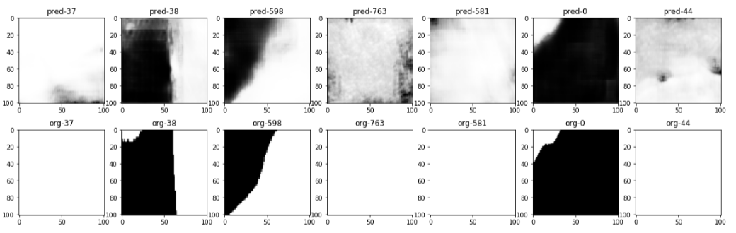
It seems that we are pretty on track. :]] Now we are moving to our final step -- IoU scoring.
Scoring by Intersection over Union (IoU)
Intersection over Union (IoU) is an evaluation metric to measure the accuracy of our object detection. It is defined by: IoU = Area of Intersection / Area of Union The "Area of Intersection" is the area where our predicted image overlaps the ground truth image (the actual "salt mask"). While the "Area of Union" is the area combining our predicted image and the ground truth image.
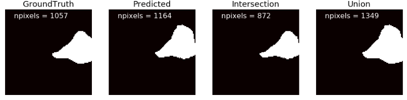
(image source, https://www.kaggle.com/pestipeti/explanation-of-scoring-metric )
From above images, the IoU is 872 / 1349 = 0.6464. A more accurate detection will have a value toward 1.
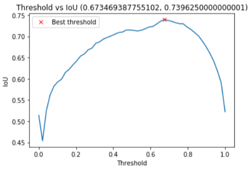
Since our predicted images are stored in single channel and normalized between 0 and 1 values. We can adjust our image threshold to find the best IoU value.
thresholds = np.linspace(0, 1, 50) # iou_metric_batch src: https://www.kaggle.com/aglotero/another-iou-metric ious = np.array([iou_metric_batch(org_valid, np.int32(preds_valid > threshold)) for threshold in tqdm(thresholds)])
We can plot a Threshold and IoU XY chart for the best threshold choice.
threshold_best_index = np.argmax(ious) iou_best = ious[threshold_best_index] threshold_best = thresholds[threshold_best_index] plt.plot(thresholds, ious) plt.plot(threshold_best, iou_best, "xr", label="Best threshold") plt.xlabel("Threshold") plt.ylabel("IoU") plt.title("Threshold vs IoU ({}, {})".format(threshold_best, iou_best)) plt.legend()
Get the Predictions
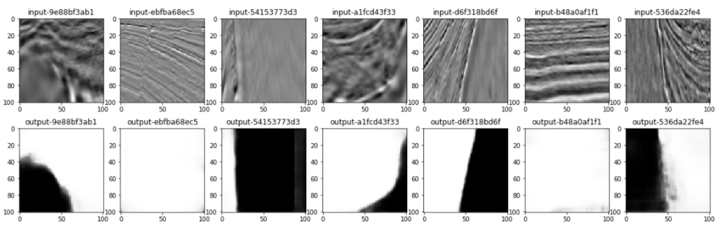
Now we can get the predictions from our U-Net model. X_test = np.array(df_test.image_array.map(upsample).tolist()).reshape(-1, targe_width, targe_height, image_channel) predict_test = (model.predict(X_test)).reshape(-1, targe_width, targe_height) And visualize our predictions. for row in range(0,row_size): image_index = 0 for col in range(0,col_size): if (row==0): img = load_img(test_image_path_array[rand_id_array[image_index]]) axundefined [col].imshow(img) title_prefix = "input" else: axundefined [col].imshow(predict_test[rand_id_array[image_index]], cmap="Greys") title_prefix = "output" axundefined [col].set_title("{}-{}".format(title_prefix, test_id_array[rand_id_array[image_index]])) image_index += 1 plt.show() Images on the first row are inputs from testing data set and images on second row are our predictions:
Export outputs to a csv file using the best threshold value for submission. predict_set = {idx: RLenc(np.round(predict_test[i]) > threshold_best ) for i, idx in enumerate(tqdm(df_test.id.values))} sub = pd.DataFrame.from_dict(predict_set,orient='index') sub.index.names = ['id'] sub.columns = ['rle_mask'] sub.to_csv('submission.csv')
Conclusion
We can get ~0.71x score (i.e. 71.x% accuracy) using above codes. There is still a lot of room for improvement, likes using pre-trained model, residual networks, test time augmentation, cross validation, etc. A better model should get at least 0.8 on scoring. The codes in this post won't provide you a high scoring model, but it provides you the fundamental knowledge on object detection. So we can understand the basic and learn to apply improvement based on it.
What have we learnt in this post?
- Architecture of U-Net
- Usage of IoU metric