TFIDF technique and Deal Probability Prediction (in Russian)

Our topic this time is too Russia, so my water just turned into Vodka :]] . Actually, this is all about Kaggle’s competition: Avito Demand Prediction Challenge. Avito is the biggest classified site in the Mother Russia, just likes the Craigslist. Our mission for this time is, predicting the rate that a seller can make a deal on Avito and handle text features with TFIDF.

Let’s get started – Load & Know

Likes the way we did on previous machine learning challenges (Titanic Survivors, Iowa House Pricing and TalkingData Click Fraud), the first thing we should do after getting the dataset is, take a look on it. Although it sounds dumb, it is just the right thing we should do. So we can make sure we load the right dataset and know what is the dataset about.

import pandas as pd 
import gc

train_df = pd.read_csv("../input/train.csv", parse_dates=["activation_date"])
train_df.head()

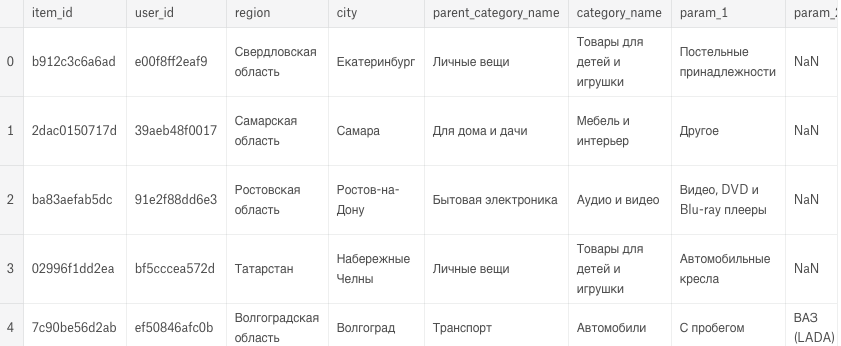
Russian, Russian, ру́сский язы́к! We also load “activate_date” as a date column, so we can apply date functions on it.

The second thing we should do is finding missing data inside the dataset.

import matplotlib.pyplot as plt
import seaborn as sns

df_missing = train_df.isnull().sum()
df_missing = df_missing[df_missing > 0]
df_missing = df_missing.append(pd.Series([train_df.shape[0]], index=['total_ads']))

plt.figure(figsize=(10,6))
sns.set_style("darkgrid")
sns.barplot(x=df_missing.values, y=df_missing.index)
plt.title("Features with Null value and Number of Total Ads")
plt.show()

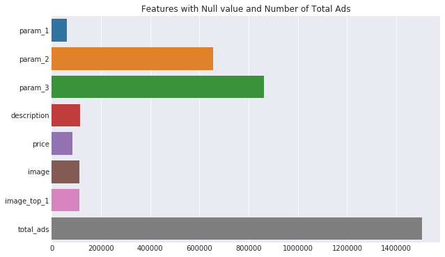
So we can think rather we need to take action on features with null value. From the top chart, we find several null features, null value in image, price and optional parameters are understandable, but what about ads without description? Let’s find out.

desc_dp = [train_df[train_df['description'].notna()]['deal_probability'].mean(), 
           train_df[train_df['description'].isna()]['deal_probability'].mean(), 
           train_df['deal_probability'].mean()]
plt.title("Deal Probability with or without description")
ax = sns.barplot(x=["With Description", "Without Description", "All Items"], y=desc_dp)
for p in ax.patches:
   ax.annotate('{:.5f}'.format(p.get_height()), (p.get_x()+p.get_width()/4, p.get_height()+.001))
plt.show

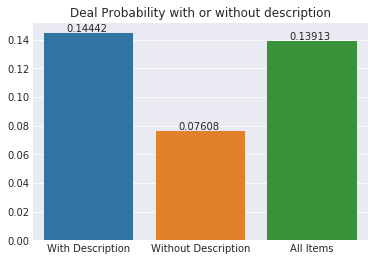
It is clear that ads without description will get lower deal probability. We can also note that description is a major feature of our challenge this time.

Interact with charts

Since we load the “activate_date” as a date object, we can create new date features from it.

train_df['weekday'] = train_df.activation_date.dt.weekday
train_df['day'] = train_df.activation_date.dt.day
train_df['week'] = train_df.activation_date.dt.week 

We can create a bar chart to show the number of ads by weekdays, but this time, we make a chart that we can interact with.

Other than our usual way to create charts with Matplotlib and Seaborn, we can now create interactive charts by Plotly.

From our Juypter notebooks (or Kaggle’s kernels), let’s import Plotly’s libraries:

import plotly.graph_objs as go
import plotly.offline as py
py.init_notebook_mode(connected=True)

Please note that “plotly.offline” module is initialized, so we can plot and save our charts locally. Then we fill up the data (number of ads by weekdays) and define the chart’s layout:

def generateBarChart(df, group_by, title, 
                     x_axis, y_axis, color="royalblue", 
                     width=700, height=400, record_size=100): 
    df2 = df.groupby([group_by]).size()[:record_size]
    
    trace = go.Bar(
            x = df2.index,
            y = df2.values,
            marker=dict(color = color)
        )

    layout = go.Layout(
                title = title,
                xaxis=dict(
                  title=x_axis
                ),
                yaxis=dict(
                  title=y_axis
                ), 
                width = width, 
                height = height
             )
    data = [trace]
    fig = go.Figure(data=data, layout=layout)
    py.iplot(fig)
    del df2;gc.collect()

generateBarChart(train_df, "weekday", "Number of Ads by Weekdays", 
"Weekdays", "Number of Ads")

When we run above codes on Jupyter notebooks, an interactive chart will appear:

We can get more detail from the bars by pointing any one of them. And we find out, Saturday (“6” from the bar chart), has the most ads posted while Friday (“5” from the chart) has the lowest in number.

Handle the Text Features

Since we know that description is an important feature affecting the deal probability, we would like to deal with it. Unlike other simple text features such as location and category, which we can encode them into numeric values. There are complex structures and varieties inside the description feature. Although we can’t simply handle the description feature, it doesn’t mean we can’t handle it at all.

Firstly, we can get the length of description of each ad.

train_df['description'] = train_df['description'].fillna(" ")
train_df['description_len'] = train_df['description'].apply(lambda x : len(x.split()))

Then we can have a look of ads with 0 to 50 words in description.

generateBarChart(train_df, "description_len", "Number of Ads for Description with (0 - 50) words", 
                    "Description length", "Number of Ads", color="lightgreen", 
                width=800, height=500, record_size=50)

Other than ads with null description, ads are trended to have 3 to 11 words in description.

Besides the word count, we can also create new textual features, like character count, punctuation count and stop words count.

import string
from nltk.corpus import stopwords

punctuation = string.punctuation
stop_words =  stopwords.words('russian')    #Avito is a Russian classified site
train_df['punctuation_count'] = train_df['description'].apply(lambda x: len("".join(_ for _ in x if _ in punctuation))) 
train_df['stopword_count'] = train_df['description'].apply(lambda x: len([wrd for wrd in x.split() if wrd.lower() in stop_words]))

We can apply the same techniques on “title”, “param_1”, “param_2” and “param_3” features. Then we can encode other categorical features like “region”, “city”, “parent_category_name”, “category_name” into numerical features.

cat_vars = ["user_id", "region", "city", "parent_category_name", "category_name", "user_type", "param_1", "param_2", "param_3"]

for col in cat_vars:
    lb = preprocessing.LabelEncoder()
    lb.fit(list(train_df[col].values.astype('str')) + list(test_df[col].values.astype('str')))
    train_df[col+'_code'] = lb.transform(list(train_df[col].values.astype('str')))
    test_df[col+'_code'] = lb.transform(list(test_df[col].values.astype('str')))

Once we have all categorical features changed to numerical features, it is time to remove those categorical features. Before doing this, let’s keep the “description” feature in another dataframe, “train_desc”. (We will explain it later)

train_desc = train_df["description"]

cols_to_drop = ["item_id", "user_id", "region", "city", "parent_category_name",  
                "category_name", "param_1", "param_2", "param_3", "title",
                "description", "activation_date", "user_type", "image", "param_combined"]            
train_df = train_df.drop(cols_to_drop, axis=1)

Now we have all numerical features, the next thing we want to know is, which features are important to deal probability? Well, we can find our answer by using a heatmap.

data = [
    go.Heatmap(
        z = train_df.corr().values,
        x = train_df.columns.values,
        y = train_df.columns.values,
        colorscale='Blackbody')
]

layout = go.Layout(
    title ='Correlation of Features',
    xaxis = dict(ticks='outside'),
    yaxis = dict(ticks='outside' ),
    width = 800, height = 700)

fig = go.Figure(data=data, layout=layout)
py.iplot(fig)

Here we go:

We know that “description” is an important feature, but we cannot find how the length and stop words features correlate with the deal probability. On the other hand, the encoded textual features, “param_1_code”, “param_2_code”, “param_3_code” and their related features have stronger correlation with deal probability. It would be good if we have a way to encode the content of “description”, so we have…

TF;IDF

No, it is not tl;dr. TFIDF stands for Term Frequency–Inverse Document Frequency. It is a weighting technique commonly used in information retrieval and text mining.

• TF (Term Frequency) is simple the count of a term appearing in a document, i.e. TF = (number of times term T appearing in a document) / (total number of terms in the document)
• IDF (Inverse Document Frequency) is the way to find out a term’ specificity among other documents, i.e. IDF = log( total number of documents / number of documents containing term T)

For example, we pick a post from this web site, and find the term “code” appearing 8 times in a post with 1000 terms. i.e. We have TF = 8 / 1000 = 0.008. Then we have 50 posts with 25 posts containing the term “code”, so we have IDF = log (50 / 25) = 0.301. At the end, the weighting of “code” is TF x IDF = 0.008 x 0.301 = 0.002408 .

So our mission is to find out the TFIDF values of words inside the textual features (in our case, “description”, “title”, “param” features).

TFIDF Transformer

First, as usual, we import required modules for TFIDF.

from sklearn.feature_extraction.text import TfidfVectorizer
from scipy.sparse import hstack, csr_matrix

We have “TfidVectorizer”, the transformer we need to get TFIDF values from textual features. Then we can assign TFIDF parameters to it and start training it.

tfidf_para = {
    "stop_words": stop_words,
    "analyzer": 'word',   #analyzer in 'word' or 'character' 
    "token_pattern": r'\w{1,}',    #match any word with 1 and unlimited length 
    "sublinear_tf": True,    #Apply sublinear tf scaling, to reduce the range of tf with 1 + log(tf)
    "dtype": np.float32,   #return data type 
    "norm": 'l2',     #apply l2 normalization
    "smooth_idf":False,   #no need to one to document frequencies to avoid zero divisions
    "ngram_range" : (1, 2),   #the min and max size of tokenized terms
    "max_features": 17000    #the top 17000 weighted features
}

tfidf_vect = TfidfVectorizer(**tfidf_para)

Do you remember the dataframe “train_desc” that we kept it a few moments ago? It is the time we transform it into TFIDF values.

tfidf_vect.fit(training_desc)

transformed_txt = tfidf_vect.transform(training_desc)

We have the “transformed_txt”, then what is that actually? It is a matrix storing the TFIDF values with 17000 (the “max_features” we set previouly) terms we gathered from “description” features. Let’s have a sneak peek on the TFIDF features.

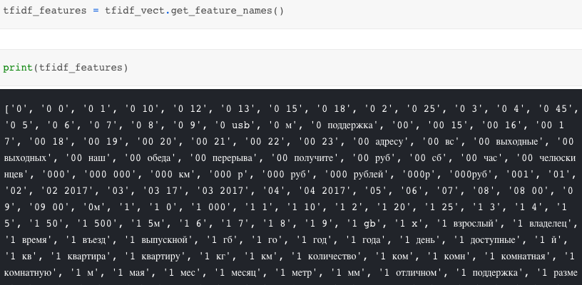
Those 17000 features contain 1 or 2 terms (from the “ngram_range” setting) and have different TFIDF values among each record. We can now integrate the training dataframe “train_df” with the TFIDF values “transformed_txt”. Since “transformed_txt” is stored as compressed sparse row matrix (CSR matrix), we have to convert “train_df” to CSR matrix then merge with “transformed_txt”.

from scipy.sparse import hstack, csr_matrix

combined_train = hstack([csr_matrix(train_df.values),transformed_txt])
combined_feat = train_df.columns.tolist() + tfidf_features

print(combined_train.shape)

After the integration, we have a dataframe with 17025 features (the original 25 features plus the 17000 TFIDF features).

(1503424, 17025)

Then we can use LGB to fit and predict the deal probability.

import lightgbm as lgb

lgb_train = lgb.Dataset(combined_train, train_df.deal_probability,
                    feature_name=combined_feat)

lgb_classifier = lgb.train(
        lgb_para,
        lgb_train,
        num_boost_round=2500,
        verbose_eval=100
    )

lgb_prediction = lgb_classifier.predict(test_df)

Please note that we only deal with one of the textual features (“description”) and limit the number of TFIDF features at 17000. It is just barely enough to run on Kaggle 17 GB RAM kernel with LGB. So if we want more accurate results, we need to invest more on our platform.

What have we learnt in this post?

1. Usage of interactive Plotly chart
2. TFIDF Handling of textual feature
3. The limitation of Kaggle free kernel