Click Fraud Detection with Machine Learning

Up to now, we have tried 3 different Kaggle journeys, the Titanic Survivors, the Iowa House Prices and the hand written digits recognition. Those journeys covered popular Machine Learning topics, such as classification, regression, deep learning, and so on. I would suggest fans of Machine Learning to start with those journeys. So we can learn the basics of Machine Learning there. After that, we can move one step further, to try a real Kaggle competition — TalkingData AdTracking Fraud Detection Challenge.

The Happy “Farm”

TalkingData is the China’s largest big data service platform, which covers 70% of active mobile devices nationwide (yeah, Big Brother is watching you :]] ). They handle 3 billion clicks a day and 90% of them are possibly fraud. In case you don’t know, there are “click farms” in China, which produce fake ratings and fake download rates.

(Click farm in China, image source: English Russia)

This Kaggle challenge is aimed to handle the click fraud issue. So our objective here is clear: build a model to determine a click is fake or not.

Click Fraud Big Data

Like our usual Data Science project routine, we read the data description, then start to load the training data and have a look on the content. Oh, wait, just know that we are handling a “big data”. A really big big data. As the training dataset contains 200 million records there! You probably need a machine with at least 32GB ram to load the entire training csv file. But what if we don’t have a decent machine? You can pay to use Amazon Web Service cloud computing, or use Kaggle free kernel. Data Science should belong to everyone, so we go for the free solution from Kaggle. And there is 17GB ram available for each kernel. Well, it is still not enough to load the complete training dataset, but hey, we have other workarounds.

Take Big Part from Big Data

We can not load the full set of training data, we can still load a part of that. Assume we are going to load a training dataset “df_train“, we can  use pandas with following options:

df_train = pd.read_csv('../input/train.csv', skiprows=range(1,125000000), nrows=50000000)

Then we have loaded 50 million [ nrows=50000000 ] out of the 200 million records, starting from the 125 million th record [ skiprows=range(1,125000000) ]. It uses around 3 minutes and 3 GB ram to load the training data.

df_train.info()

RangeIndex: 50000000 entries, 0 to 49999999
Data columns (total 8 columns):
ip                 int64
app                int64
device             int64
os                 int64
channel            int64
click_time         object
attributed_time    object
is_attributed      int64
dtypes: int64(6), object(2)
memory usage: 3.0+ GB

Let’s tell our system on what columns and the data types to load:

#columns and their data types to load
dtypes = {
        'ip'            : 'uint32',
        'app'           : 'uint16',
        'device'        : 'uint16',
        'os'            : 'uint16',
        'channel'       : 'uint16',
        'is_attributed' : 'uint8',
        'click_id'      : 'uint32',
        }

columns = ['ip','app','device','os', 'channel', 'click_time', 'is_attributed']

df_train = pd.read_csv('../input/train.csv', skiprows=range(1,125000000), nrows=50000000, dtype=dtypes, usecols=columns)

And here we got:

RangeIndex: 50000000 entries, 0 to 49999999
Data columns (total 7 columns):
ip               uint32
app              uint16
device           uint16
os               uint16
channel          uint16
click_time       object
is_attributed    uint8
dtypes: object(1), uint16(4), uint32(1), uint8(1)
memory usage: 1001.4+ MB

It uses only 1GB ram to load the data now.

“I will DELETE you!”

Another tip on memory tight environment is, delete AND garbage collect every unused segment. Although there is automatic garbage collection in Python, it will only run when the ratio of allocations / deallocations hits the threshold. In this case, we can run the garbage collection manually to free memory blocks.

import gc
del df_train
gc.collect()

EDA on the Click Fraud data set

Now we have the training data, it is time to run our EDA (exploratory data analysis) on the click industry. The challenge is about finding the fraud rate, so the first thing I would like to know is, how “fake” of those clicks are in the training data? i.e. What is the percentage of a click leading to an app download?

download_rate = df_train['is_attributed'].value_counts(normalize=True)*100
ax = sns.barplot(['Click without download', 'Click with download'], download_rate)
for p in ax.patches:
    ax.annotate('{:.2f}%'.format(p.get_height()), (p.get_x()+p.get_width()/3, p.get_height()+0.1))

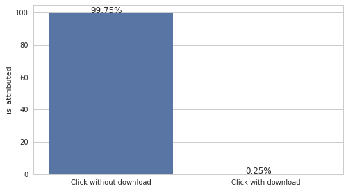
About 99.75% of clicks are fraud. (For lazy data scientists: just fill up your output file with 0.0025, then the work is done :]] )

Let’s check out the unique values per feature in our training data:

cols = ['ip', 'app', 'device', 'os', 'channel']
uniques = [len(df_train[col].unique()) for col in cols]
ax =sns.barplot(cols, uniques, log=True)
for p in ax.patches:
    ax.annotate(p.get_height(), (p.get_x()+p.get_width()/3, p.get_height()+0.1))

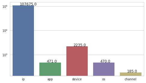
As expected, ip address is the largest feature with unique values, while channel is the one with fewer unique values. So we can see ‘channel’ taking a big part in our machine learning model.

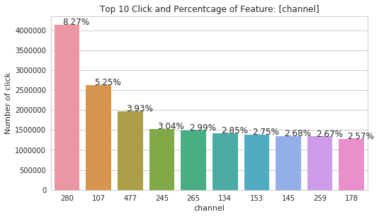
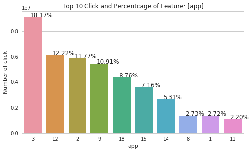
And we take a look on the distribution of our features, first, we go for ‘channel’.

def displayCountAndPercentage(df, groupby, countby):
    counts = df[[groupby]+[countby]].groupby(groupby, as_index=False).count().sort_values(countby, ascending=False)
    percentage = df[groupby].value_counts(normalize=True)*100
    ax = sns.barplot(x=groupby, y="is_attributed", data=counts[:10], order=counts[groupby][:10])
    ax.set(ylabel='Number of click', title='Top 10 Click and Percentcage of Feature: [{}]'.format(groupby))

    i = 0
    for p in ax.patches:    
        ax.annotate('{:.2f}%'.format(percentage.iloc[i]), (p.get_x()+p.get_width()/3, p.get_height()+0.5))
        i = i + 1

    del counts, percentage
    gc.collect()  

displayCountAndPercentage(df_train, 'channel', 'is_attributed')

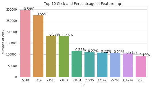
After that, we use the same function on ‘ip’, ‘app’, ‘os’ and ‘device’ features.

 
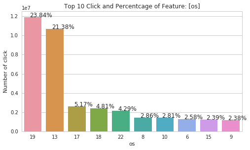
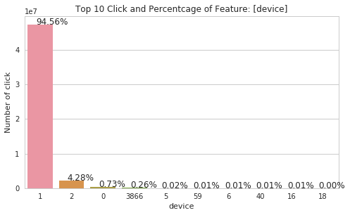
There are interesting plots on ‘os’ and ‘device’ features. As those features are dominated by certain values. The ‘device’ feature is dominated by the encoded value ‘1’ with 94.56%. And we are pretty sure that the ‘1’ device is Android and the ‘2’ device is iPhone. So we can also assume os ’19’, ’13’, ’17’, ’18’ and ’22’ are all Android OS in different versions.

Relationship between Number of Click and Download Rate

We know certain values dominated a feature, but how do they take part in the download rate? Let’s find it out. This time, we take a look on the top 20 clicks in each feature, and see how they perform in term of download rate. We go for the ‘device’ feature first this time.

def displayCountAndDownloadRate(df, groupby, countby, top):
   counts = df[[groupby]+[countby]].groupby(groupby, as_index=False).count().sort_values(countby, ascending=False)       
   download_rates = df[[groupby]+[countby]].groupby(groupby, as_index=False).mean().sort_values(countby, ascending=False)
   df_merge = counts.merge(download_rates, on=groupby, how='left')
   del counts,download_rates
   gc.collect()
   df_merge.columns = [groupby, 'click_count', 'download_rate']
   df_merge[groupby] = df_merge[groupby].astype('category')
   ax = df_merge[:top].plot(x=groupby, y="download_rate", legend=False, kind="bar", color="orange", label="download rate (left)")
   ax2 = ax.twinx()
   df_merge[:top].plot(x=groupby, y="click_count", ax=ax2, legend=False, kind="line", color="blue",  label="click count (right)")
   ax.set_xticklabels(df_merge[groupby])
   ax.figure.legend(loc='upper left')
   ax.set_title("Top {} Click Counts and Download Rates of [{}]".format(top, groupby)) 
   del df_merge
   gc.collect() 

displayCountAndDownloadRate(df_train, 'device', 'is_attributed', 20)

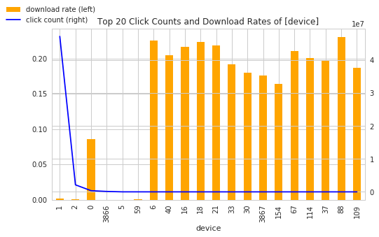
Device “1” and “2” take 99+% of all devices, but their download rates are around 0.0017 (0.17%) and 0.00029 (0.029%). Other uncommon devices can get 15%+ download rates, but they are lower than 1% of the data. (Lazy scientists part 2: let’s fill 95% of output file with 0.0018 )

Again, we apply the same function on ‘os’, ‘ip’, ‘channel’ and ‘app’ features.

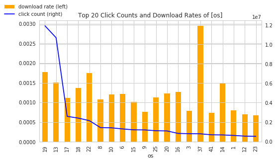
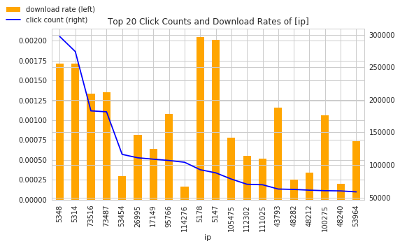
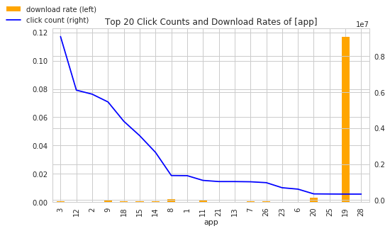
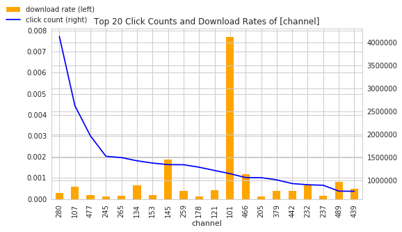
There are some findings from above charts: Android OSes hardly make an impact on download rate, it matches our observation on Top device Click/Download rate chart. The top 20 ip clickers did download! Although their download rates are tiny, a download is a download, we can’t write off them for being big clickers. For channel and app, the download rate does not correlate the number of clicks much. Certain apps and channels just out-download others, no matter the size of clicks.

Does Time matter?

Since there are massive clicks and the download rate is low in general, we are making 2 assumptions:

1. clicks came from hired clickers
2. clicks came from click flooding

As of 2017 November (the training data record date), click farm and click flooding are still the major players in click fraud (reference: The State of Mobile Fraud: Q1 2018). Click farm companies should hire click farmers and operate click flooding in regular working hours to control the cost, i.e. around 0900 to 1800. The usage of click bots in non-office hours is omitted, as the use of bots in mobile fraud was still low in 2017. Then we take a look on the click time distribution. But first, since those click time records in training data are in UTC, we have to convert them to China time, i.e. GMT +8. After that, we round those click time records to nearest hour.

df_train['click_time_china'] = pd.to_datetime(df_train.click_time)
df_train['click_time_china'] += pd.to_timedelta(8, unit='h')
df_train['click_time_hour']=pd.to_datetime(df_train['click_time_china']).dt.round('H') 

And get the click counts and download rates in 24 hours.

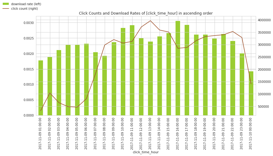
According to eMarketer report, 2100 to 2359 should be the peak section for Chinese mobile users. Then we have even more counts then the peak hours during 1200 to 1500. It matches our assumption of click farm companies’ operation in office hours. We may need to add a new feature, “farm_hour”, to indicate a time period with higher click farming activity.

The Next Steps

There is more than one way to do feature engineering for the TalkingData challenge. You may create a new feature which combines ip and device or app and channel. Or create a feature which indicates the next or previous click of a user. After that, you can pick a learning model to predict your results.

For starter, you can take a look of my Random Forest kernel here. It won’t help you to get high score in leaderboard (use LGB if you are looking for higher score), but it is easy to understand and straight forward. In case you don’t know, I am always a fan of Random Forest model :]] .

Just use what you have learnt to process the results, don’t be afraid of failing. Every time we fail, get up and see what we have done wrong. Then we can learn from mistakes and become better and better.

 

What have we learnt in this post?

1. Handle large data set with limited resources
2. Use charts on EDA (Exploratory Data Analysis)
3. Don’t be afraid of failing!